Spin and polarization

The spin of the particles can be tracked in Xsuite together with the other 6D phase space coordinates. Additionally, the twiss module can provide the spin closed solution and the equilibrium polarization due to the Sokolov-Ternov effect.

Equilibrium polarization and spin closed solution

In the following example the twiss module is used to compute the effect of solenoid and compensation bumps on the spin closed solution and on the equilibrium polarization in the LEP collider.

import xtrack as xt
import matplotlib.pyplot as plt

# Load LEP lattice
line = xt.load('../../test_data/lep/lep_sol.json')

# Make sure anomalous magnetic moment is set:
line.particle_ref.anomalous_magnetic_moment # is 0.00115965

# Set solenoids and compensation bumps off
line['on_solenoids'] = 0
line['on_spin_bumps'] = 0
line['on_coupling_corrections'] = 0

# Twiss with spin and polarization calculation
tw_no_sol = line.twiss4d(spin=True, polarization_analysis=True)

# Inspect equilibrium polarization
tw_no_sol.spin_polarization_eq # is 0.92376

# Enable solenoids and corresponding coupling corrections
line['on_solenoids'] = 1
line['on_spin_bumps'] = 0
line['on_coupling_corrections'] = 1

# Twiss with spin and polarization calculation
tw_sol = line.twiss4d(spin=True, polarization_analysis=True)

# Inspect equilibrium polarization
tw_sol.spin_polarization_eq # is 0.018617

# Enable also spin bumps
line['on_solenoids'] = 1
line['on_spin_bumps'] = 1
line['on_coupling_corrections'] = 1

# Twiss with spin and polarization calculation
tw = line.twiss4d(spin=True, polarization_analysis=True)

# Inspect equilibrium polarization
tw.spin_polarization_eq # is 0.89160

# Plot spin closed solution (n_0)
plt.figure(figsize=(6.4, 4.8*1.3))
ax1 = plt.subplot(3, 1, 1)
tw.plot('y', ax=ax1)
ax2 = plt.subplot(3, 1, 2)
tw.plot('spin_x spin_z', ax=ax2)
plt.ylabel(r'$n_{0,x}, n_{0,z}$')
ax3 = plt.subplot(3, 1, 3, sharex=ax1)
tw.plot('spin_y', ax=ax3)
plt.ylabel(r'$n_{0,y}$')
plt.ylim(0.998, 1.001)

plt.show()

# Complete source: xtrack/examples/spin_lep/001_n0_and_eq_polarization.py

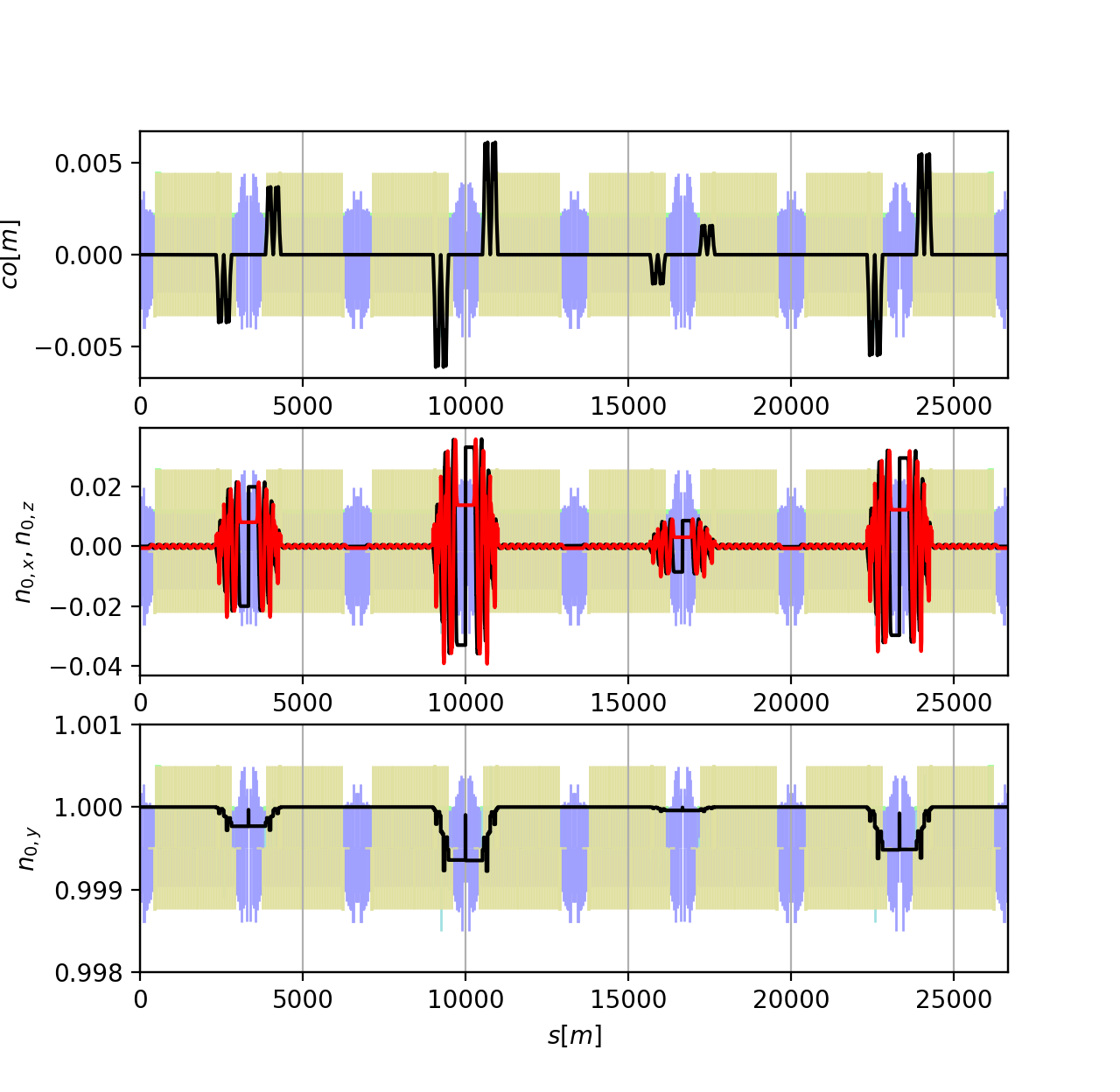
The spin closed solution from the example above.

Tracking with spin and Monte Carlo simulation of radiative depolarization

The following example shows how, by tracking particles with spin and including synchrotron radiation and quantum excitation, one can simulate the radiative depolarization in the LEP collider. This method, which accounting for non-linear effects in the estimation of the equilibrium polarization, is described in detail in Z. Duan et al., A Monte-Carlo simulation of the equilibrium beam polarization in ultra-high energy electron (positron) storage rings .

import xtrack as xt
import xpart as xp
import xobjects as xo
import numpy as np
from scipy.stats import linregress
import matplotlib.pyplot as plt

# Some references:
# CERN-SL-94-71-BI https://cds.cern.ch/record/267514
# CERN-LEP-Note-629 https://cds.cern.ch/record/442887

# Load and configure ring model
line = xt.Line.from_json('../../test_data/lep/lep_sol.json')
line['vrfc231'] = 12.65  # RF voltage -> qs=0.6 with radiation

# Match tunes to those used during polarization measurements
# https://cds.cern.ch/record/282605
opt = line.match(
    method='4d',
    solve=False,
    vary=xt.VaryList(['kqf', 'kqd'], step=1e-4),
    targets=xt.TargetSet(qx=65.10, qy=71.20, tol=1e-4)
)
opt.solve()

# Solenoids and spin compensation bumps
line['on_solenoids'] = 1
line['on_spin_bumps'] = 1
line['on_coupling_corrections'] = 1

# Enable radiation (mean mode)
line.configure_radiation('mean')

# Generate a matched bunch distribution
tw = line.twiss(spin=True, radiation_analysis=True, polarization_analysis=True)
np.random.seed(0)
particles = xp.generate_matched_gaussian_bunch(
    line=line,
    nemitt_x=tw.eq_nemitt_x,
    nemitt_y=tw.eq_nemitt_y,
    sigma_z=np.sqrt(tw.eq_gemitt_zeta * tw.bets0),
    num_particles=300)
# Add stable phase
particles.zeta += tw.zeta[0]
particles.delta += tw.delta[0]

# Initialize spin of all particles along n0
particles.spin_x = tw.spin_x[0]
particles.spin_y = tw.spin_y[0]
particles.spin_z = tw.spin_z[0]

# Simulate bunch evolution with stochastic photon emission
line.configure_spin('auto')
line.configure_radiation(model='quantum')

# Enable parallelization
line.discard_tracker()
line.build_tracker(_context=xo.ContextCpu(omp_num_threads=10))

# Track
num_turns=200
line.track(particles, num_turns=num_turns, turn_by_turn_monitor=True,
           with_progress=10)
mon = line.record_last_track


# Fit depolarization time
mask_alive = mon.state > 0
pol_x = mon.spin_x.sum(axis=0)/mask_alive.sum(axis=0)
pol_y = mon.spin_y.sum(axis=0)/mask_alive.sum(axis=0)
pol_z = mon.spin_z.sum(axis=0)/mask_alive.sum(axis=0)
pol = np.sqrt(pol_x**2 + pol_y**2 + pol_z**2)

i_start = 3 # Skip a few turns (small initial mismatch)
pol_to_fit = pol[i_start:]/pol[i_start]

turns = np.arange(len(pol_to_fit))
slope, intercept, r_value, p_value, std_err = linregress(turns, pol_to_fit)
# Calculate depolarization time
t_dep_turns = -1 / slope

# Plot polarization decay and fit
plt.figure()
plt.plot(pol_to_fit-1, label='Tracking')
plt.plot(turns, intercept*np.exp(-turns/t_dep_turns) - 1, label='Fit')
plt.ylabel(r'$P/P_0 - 1$')
plt.xlabel('Turn')
plt.subplots_adjust(left=.2)
plt.legend()

# Compute equilibrium polarization
p_inf = tw['spin_polarization_inf_no_depol']
t_pol_turns = tw['spin_t_pol_component_s']/tw.t_rev0

p_eq = p_inf * 1 / (1 + t_pol_turns/t_dep_turns)
# gives 0.853721

# Complete source: xtrack/examples/spin_lep/002a_monte_carlo_polarization.py

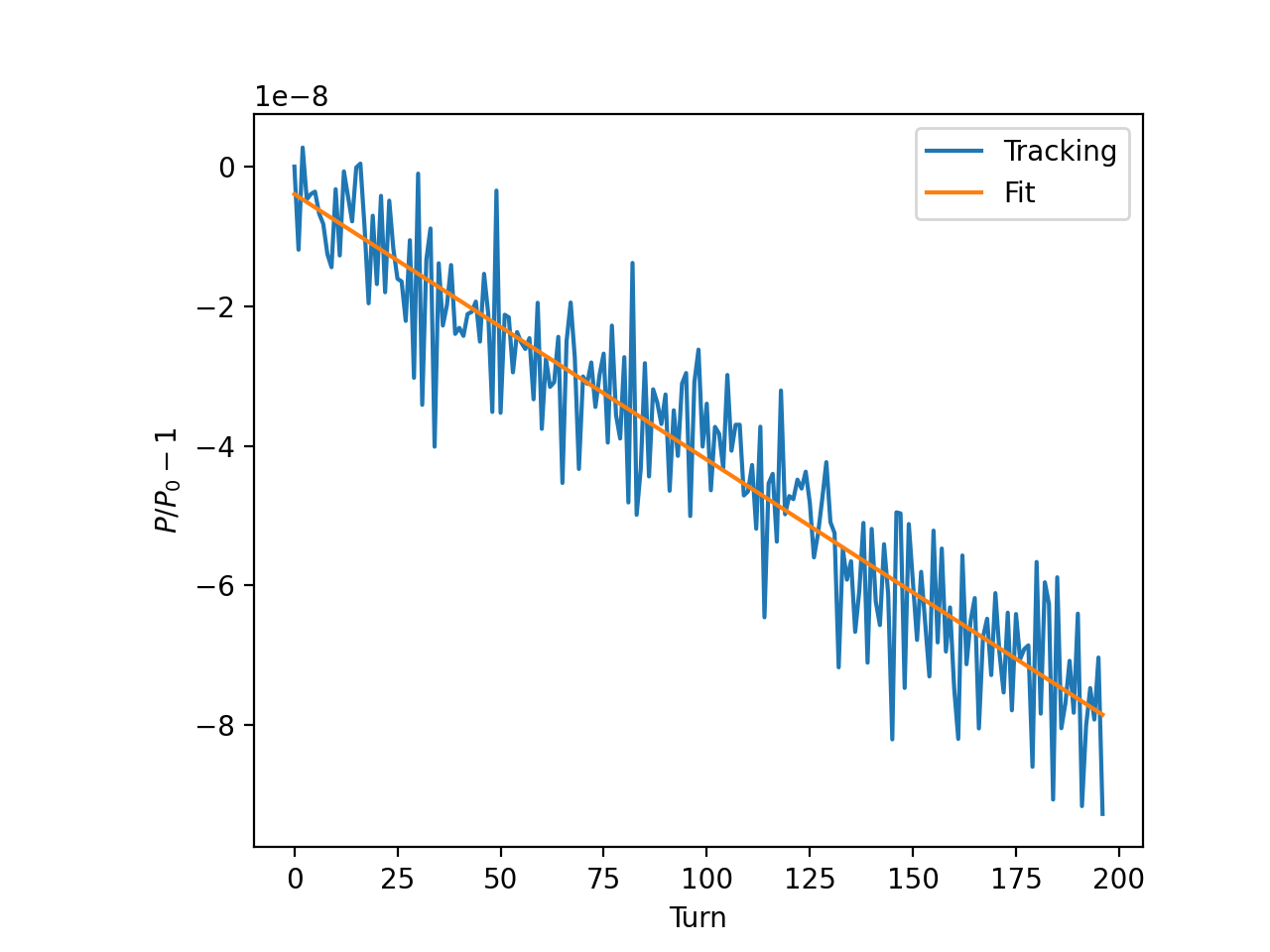
The polarization decay from the Monte Carlo simulation (blue dots) and the fitted exponential decay (orange line).