Twiss
Xtrack provides a twiss method associated to the line that can be used to obtain the lattice functions and other quantities like tunes, chromaticities, slip factor, etc. This is illustrated in the following examples. For a complete description of all available options and output quantities, please refer to the Twiss API reference.
See also TwissTable class in the Reference
guide for the table type returned by line.twiss().
Basic usage (ring)
The following example shows how to use the twiss method to obtain the lattice functions and other quantities for a ring.
import numpy as np
import xtrack as xt

# Load a line
line = xt.load('../../test_data/hllhc15_thick/lhc_thick_with_knobs.json')
line.set_particle_ref('proton', energy0=7e12)
line['vrf400'] = 16 # set rf voltage

# Twiss
tw = line.twiss()

# Inspect tunes and chromaticities
tw.qx # Horizontal tune
tw.qy # Vertical tune
tw.dqx # Horizontal chromaticity
tw.dqy # Vertical chromaticity

# Plot closed orbit and lattice functions
import matplotlib.pyplot as plt
plt.close('all')

fig1 = plt.figure(1, figsize=(6.4, 4.8*1.5))
spbet = plt.subplot(3,1,1)
spco = plt.subplot(3,1,2, sharex=spbet)
spdisp = plt.subplot(3,1,3, sharex=spbet)

spbet.plot(tw.s, tw.betx)
spbet.plot(tw.s, tw.bety)
spbet.set_ylabel(r'$\beta_{x,y}$ [m]')

spco.plot(tw.s, tw.x)
spco.plot(tw.s, tw.y)
spco.set_ylabel(r'(Closed orbit)$_{x,y}$ [m]')

spdisp.plot(tw.s, tw.dx)
spdisp.plot(tw.s, tw.dy)
spdisp.set_ylabel(r'$D_{x,y}$ [m]')
spdisp.set_xlabel('s [m]')

fig1.suptitle(
    r'$q_x$ = ' f'{tw.qx:.5f}' r' $q_y$ = ' f'{tw.qy:.5f}' '\n'
    r"$Q'_x$ = " f'{tw.dqx:.2f}' r" $Q'_y$ = " f'{tw.dqy:.2f}'
    r' $\gamma_{tr}$ = '  f'{1/np.sqrt(tw.momentum_compaction_factor):.2f}'
)

fig1.subplots_adjust(left=.15, right=.92, hspace=.27)
plt.show()

# Complete source: xtrack/examples/twiss/000_twiss.py
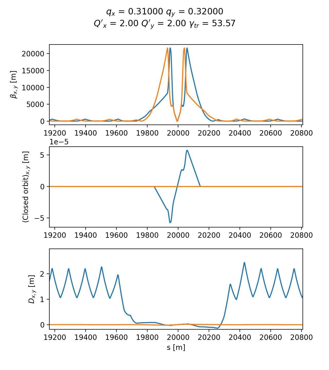
Lattice functions and accelerator parameters as obtained by Xtrack twiss.
Inspecting twiss output
The twiss table has several access options as illustrated in the following example.
import numpy as np

import xtrack as xt

# Load a line
line = xt.load('../../test_data/hllhc15_thick/lhc_thick_with_knobs.json')
line.set_particle_ref('proton', p0c=7e12)

# Twiss
tw = line.twiss(method='4d')

# Print table
tw.show()
# prints:
#
# TwissTable: 13401 rows, 70 cols
# name                     s             x            px             y ...
# ip7                      0             0             0             0
# drift_0                  0             0             0             0
# tcsg.a4r7.b1           0.5             0             0             0
# drift_1                1.5             0             0             0
# mcbwv.4r7.b1        53.341             0             0             0
# drift_2             55.041             0             0             0
# bpmw.4r7.b1        57.9855             0             0             0
# drift_3            57.9855             0             0             0
# mqwa.a4r7.b1        58.622             0             0             0
# drift_4              61.73             0             0             0
# ...
# bpmw.4l7.b1        26600.8  -4.24811e-16   3.18642e-18  -5.00664e-33
# drift_6658         26600.8  -4.24811e-16   3.18642e-18  -5.00664e-33
# mcbwh.4l7.b1       26601.5  -4.22611e-16   3.18642e-18  -5.01626e-33
# drift_6659         26603.2  -4.17194e-16   3.18642e-18  -5.03996e-33
# tcsg.b4l7.b1       26651.4  -2.63701e-16   3.18642e-18  -5.71147e-33
# drift_6660         26652.4  -2.60515e-16   3.18642e-18  -5.72541e-33
# tcsg.a4l7.b1       26655.4  -2.50955e-16   3.18642e-18  -5.76723e-33
# drift_6661         26656.4  -2.47769e-16   3.18642e-18  -5.78118e-33
# lhcb1ip7_p_        26658.9  -2.39803e-16   3.18642e-18  -5.81603e-33
# _end_point         26658.9  -2.39803e-16   3.18642e-18  -5.81603e-33

# Access to scalar quantities
tw.qx    # is : 62.31000
tw['qx'] # is : 62.31000

# Access to a single column of the table
tw['betx'] # is an array with the horizontal beta function at all elements

# Access to a single element of the table of a vector quantity
tw['betx', 'ip1'] # is 0.150000

# Regular expressions can be used to select elements by name
tw.rows['ip.*']
# returns:
#
# TwissTable: 9 rows, 41 cols
# name                           s x px y py zeta delta ptau    betx    bety ...
# ip7                            0 0  0 0  0    0     0    0 120.813 149.431
# ip8                      3321.22 0  0 0  0    0     0    0     1.5     1.5
# ip1.l1                   6664.72 0  0 0  0    0     0    0    0.15    0.15
# ip1                      6664.72 0  0 0  0    0     0    0    0.15    0.15
# ip2                      9997.16 0  0 0  0    0     0    0      10      10
# ip3                      13329.4 0  0 0  0    0     0    0 121.567 218.584
# ip4                      16661.7 0  0 0  0    0     0    0  236.18 306.197
# ip5                        19994 0  0 0  0    0     0    0    0.15    0.15
# ip6                      23326.4 0  0 0  0    0     0    0 273.434  183.74

# A section of the ring can be selected using names
tw.rows['ip5':'mqxfa.a1r5/lhcb1']
# returns:
#
# TwissTable: 8 rows, 70 cols
# name                        s             x            px ...
# ip5                     19994   5.14781e-18  -8.47233e-17
# mbcs2.1r5               19994   5.14781e-18  -8.47233e-17
# drift_5020            20000.5  -5.45553e-16  -8.47233e-17
# taxs.1r5              20013.1  -1.60883e-15  -8.47233e-17
# drift_5021            20014.9  -1.76133e-15  -8.47233e-17
# bpmqstza.1r5.b1       20015.9  -1.84783e-15  -8.47233e-17
# drift_5022            20015.9  -1.84783e-15  -8.47233e-17
# mqxfa.a1r5            20016.9   -1.9373e-15  -8.47233e-17

# A section of the ring can be selected using the s coordinate
tw.rows[300:305:'s']
# returns:
#
# TwissTable: 5 rows, 70 cols
# name                     s             x            px             y ...
# bpm.8r7.b1         300.698  -1.46744e-16  -9.41823e-18             0
# drift_52           300.698  -1.46744e-16  -9.41823e-18             0
# mq.8r7.b1          301.695  -1.56134e-16  -9.41823e-18             0
# drift_53           304.795  -1.92329e-16  -1.40959e-17             0
# mqtli.8r7.b1       304.964  -1.94711e-16  -1.40959e-17             0

# A section of the ring can be selected using indexes relative one element
# (e.g. to get from three elements upstream of 'ip5' to two elements
# downstream of 'ip5')
tw.rows['ip5<<3':'ip5>>2']
# returns:
#
# TwissTable: 6 rows, 70 cols
# name                   s             x            px             y ...
# taxs.1l5         19973.2   1.77163e-15  -8.47233e-17   5.46514e-33
# drift_5019         19975   1.61913e-15  -8.47233e-17    5.0159e-33
# mbcs2.1l5        19987.5   5.55849e-16  -8.47233e-17   1.88372e-33
# ip5                19994   5.14781e-18  -8.47233e-17   2.61468e-34
# mbcs2.1r5          19994   5.14781e-18  -8.47233e-17   2.61468e-34
# drift_5020       20000.5  -5.45553e-16  -8.47233e-17  -1.36078e-33

# Columns can be selected as well (and defined on the fly with simple mathematical
# expressions)
tw.cols['betx dx/sqrt(betx)']
# returns:
#
# TwissTable: 13401 rows, 3 cols
# name                  betx dx/sqrt(betx)
# ip7                120.813    -0.0185459
# drift_0            120.813    -0.0185459
# tcsg.a4r7.b1       119.542    -0.0186442
# drift_1            117.031    -0.0188431
# mcbwv.4r7.b1       46.5375    -0.0298815
# ...

# Each of the selection methods above returns a valid table, hence selections
# can be chained. For example we can get the beta functions at all the skew
# quadrupoles between ip1 and ip2:

tw.rows['ip1':'ip2'].rows['mqs.*b1'].cols['betx bety']
# returns:
#
# TwissTable: 4 rows, 3 cols
# name                        betx    bety
# mqs.23r1.b1              574.134 57.4386
# mqs.27r1.b1              574.134 57.4386
# mqs.27l2.b1              59.8967 62.0111
# mqs.23l2.b1              59.8968  62.011

# Complete source: xtrack/examples/twiss/017_table_slicing.py
4d method (RF off)
When the RF cavities are disabled or not included in the lattice (or when the longitudinal motion is artificially frozen) it is not possible to use the standard method for the twiss calculation. In these cases, the “4d” method can be used, as illustrated in the following examples:
import xtrack as xt

# Load a line
line = xt.load(
    '../../test_data/hllhc15_noerrors_nobb/line_and_particle.json')
line.set_particle_ref('proton', p0c=7e12)

# We consider a case in which all RF cavities are off
tab = line.get_table()
tab_cav = tab.rows[tab.element_type == 'Cavity']
for nn in tab_cav.name:
    line[nn].voltage = 0

# For this configuration, `line.twiss()` gives an error because the
# longitudinal motion is not stable.
# In this case, the '4d' method of `line.twiss()` can be used to compute the
# twiss parameters.

tw = line.twiss(method='4d')

# Complete source: xtrack/examples/twiss/008_4d_twiss_and_particle_match.py
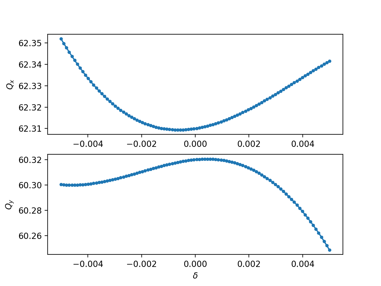
Off-momentum twiss
The 4d mode of the twiss can be used providing in input the initial momentum. This feature can be used to measure the non-linear momentum detuning of a ring as shown in the following example:
import numpy as np
from cpymad.madx import Madx

import xtrack as xt

mad = Madx()
mad.call('../../test_data/hllhc15_noerrors_nobb/sequence.madx')
mad.use('lhcb1')

line = xt.Line.from_madx_sequence(mad.sequence.lhcb1)
line.set_particle_ref('proton', p0c=7000e9)

tw = line.twiss()

delta_values = np.linspace(-5e-3, 5e-3, 100)

qx_values = delta_values * 0
qy_values = delta_values * 0
for i, delta in enumerate(delta_values):
    print(f'Xsuite working on {i} of {len(delta_values)}  ', end='\r', flush=True)
    tt = line.twiss(method='4d', delta0=delta)

    qx_values[i] = tt.qx
    qy_values[i] = tt.qy

# Complete source: xtrack/examples/twiss/011_tune_vs_delta.py
Twiss with “initial” conditions
The twiss calculation can be performed with initial conditions provided by the users or extracted from an existing twiss table, as illustrated in the following example:
import xtrack as xt

# Load a line
line = xt.load('../../test_data/hllhc15_noerrors_nobb/line_and_particle.json')
line.set_particle_ref('proton', energy0=7e12)

# Periodic twiss
tw_p = line.twiss()

# Twiss over a range with user-defined initial conditions (at start)
tw1 = line.twiss(start='ip5', end='mb.c24r5.b1',
                betx=0.15, bety=0.15, py=1e-6)


# Twiss over a range with user-defined initial conditions at end
tw2 = line.twiss(start='ip5', end='mb.c24r5.b1', init_at=xt.END,
                alfx=3.50482, betx=131.189, alfy=-0.677173, bety=40.7318,
                dx=1.22515, dpx=-0.0169647)

# Twiss over a range with user-defined initial conditions at arbitrary location
tw3 = line.twiss(start='ip5', end='mb.c24r5.b1', init_at='mb.c14r5.b1',
                 alfx=-0.437695, betx=31.8512, alfy=-6.73282, bety=450.454,
                 dx=1.22606, dpx=-0.0169647)

# Initial conditions can also be taken from an existing twiss table
tw4 = line.twiss(start='ip5', end='mb.c24r5.b1', init_at='mb.c14r5.b1',
                 init=tw_p)

# More explicitly, a `TwissInit` object can be extracted from the twiss table
# and used as initial conditions
tw_init = tw_p.get_twiss_init('mb.c14r5.b1',)
tw5 = line.twiss(start='ip5', end='mb.c24r5.b1', init=tw_init)

# Complete source: xtrack/examples/twiss/000a_twiss_range.py
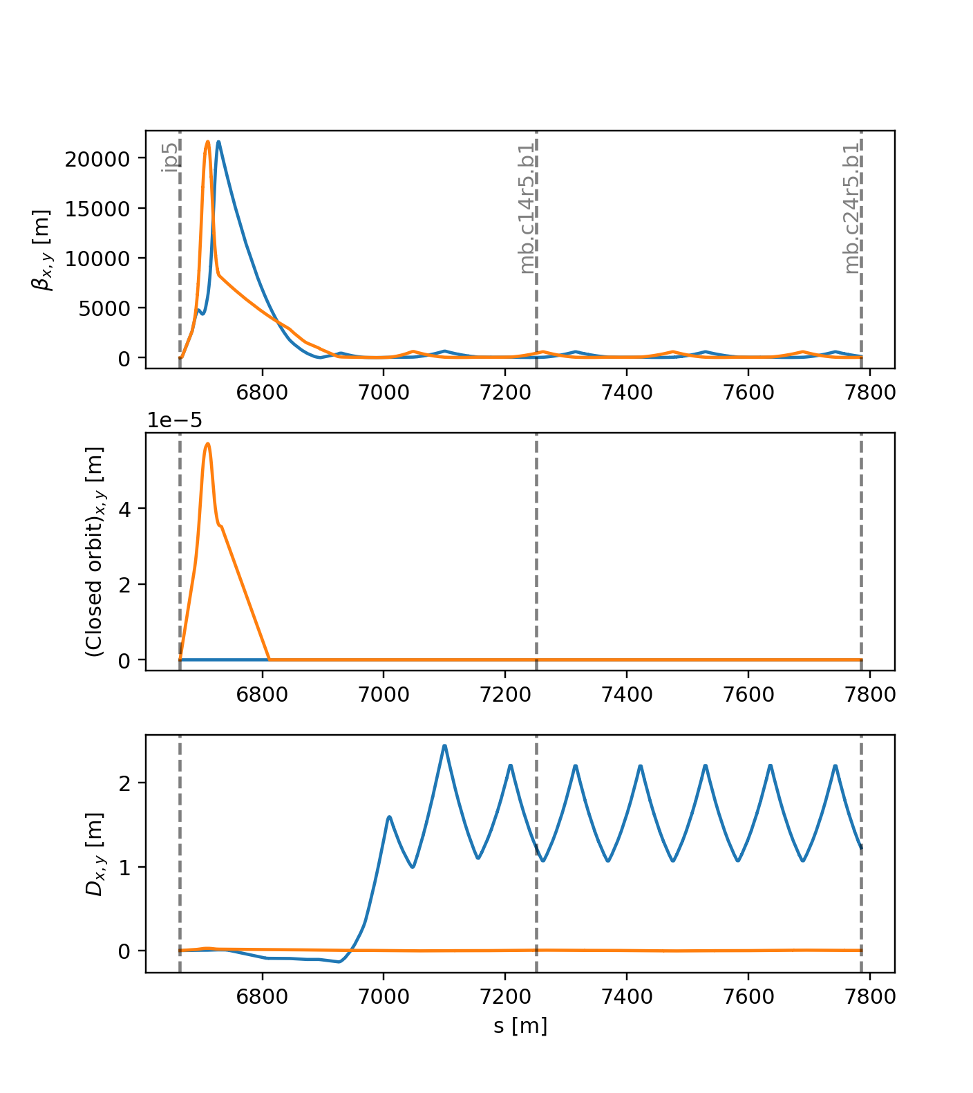
Result of all twiss calculations with initial conditions shown in the example above.
Periodic twiss on a portion of a line
The twiss method can also be used to find the periodic solution for a portion of a beam line, as illustrated in the following example:
import xtrack as xt

# Load a line
line = xt.load('../../test_data/hllhc15_noerrors_nobb/line_and_particle.json')
line.set_particle_ref('proton', energy0=7e12)

# Periodic twiss of the full ring
tw_p = line.twiss()

# Periodic twiss of an arc cell
tw = line.twiss(method='4d', start='mq.14r6.b1', end='mq.16r6.b1', init='periodic')

# Complete source: xtrack/examples/twiss/000b_twiss_range_periodic.py
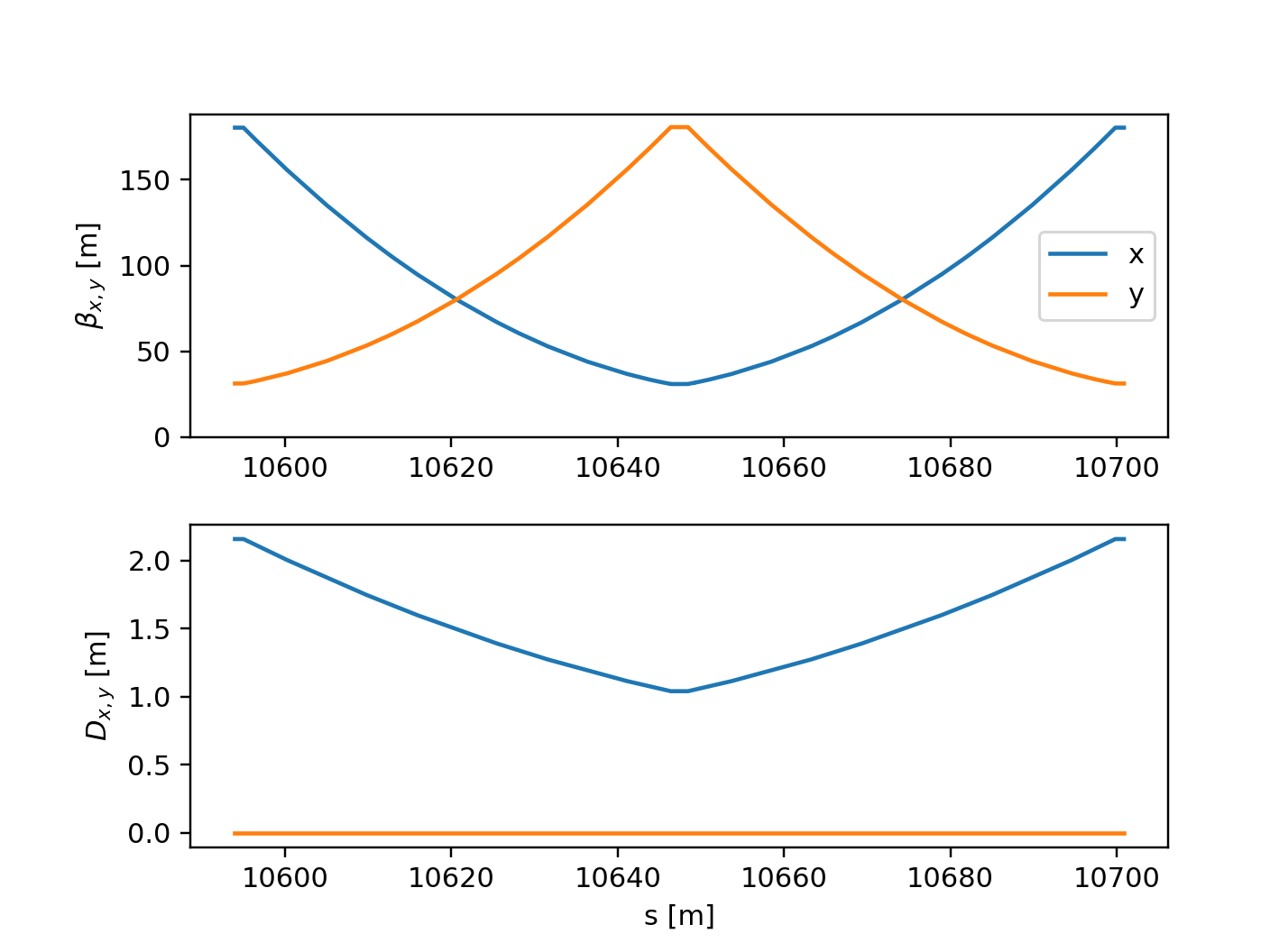
Result of the twiss with periodic boundary conditions.
Beam sizes from twiss table
The transverse and longitudinal beam sizes can be computed from the twiss table, as illustrated in the following example:
import numpy as np
import xtrack as xt

# Load a line
line = xt.load('../../test_data/hllhc15_noerrors_nobb/line_and_particle.json')
line.set_particle_ref('proton', p0c=7e12)

# Twiss
tw = line.twiss()

# Transverse normalized emittances
nemitt_x = 2.5e-6
nemitt_y = 2.5e-6

# Longitudinal emittance from energy spread
sigma_pzeta = 2e-4
gemitt_zeta = sigma_pzeta**2 * tw.bets0
# similarly, if the bunch length is known, the emittance can be computed as
# gemitt_zeta = sigma_zeta**2 / tw.bets0

# Compute beam sizes
beam_sizes = tw.get_beam_covariance(nemitt_x=nemitt_x, nemitt_y=nemitt_y,
                                    gemitt_zeta=gemitt_zeta)

# Inspect beam sizes (table can be accessed similarly to twiss tables)
beam_sizes.rows['ip.?'].show()
# prints
#
# name                       s     sigma_x     sigma_y sigma_zeta    sigma_px ...
# ip3                        0 0.000226516 0.000270642    0.19694 4.35287e-06
# ip4                  3332.28 0.000281326 0.000320321   0.196941 1.30435e-06
# ip5                  6664.57  7.0898e-06 7.08975e-06    0.19694  4.7265e-05
# ip6                  9997.01 0.000314392 0.000248136   0.196939 1.61401e-06
# ip7                  13329.4 0.000205156 0.000223772   0.196939 2.70123e-06
# ip8                  16650.7 2.24199e-05 2.24198e-05   0.196939 1.49465e-05
# ip1                  19994.2 7.08975e-06 7.08979e-06   0.196939 4.72651e-05
# ip2                  23326.6 5.78877e-05 5.78878e-05   0.196939 5.78879e-06

# All covariances are computed including those from linear coupling
beam_sizes.keys()
# is:
#
# ['s', 'name', 'sigma_x', 'sigma_y', 'sigma_zeta', 'sigma_px', 'sigma_py',
# 'sigma_pzeta', 'Sigma', 'Sigma11', 'Sigma12', 'Sigma13', 'Sigma14', 'Sigma15',
# 'Sigma16', 'Sigma21', 'Sigma22', 'Sigma23', 'Sigma24', 'Sigma25', 'Sigma26',
# 'Sigma31', 'Sigma32', 'Sigma33', 'Sigma34', 'Sigma41', 'Sigma42', 'Sigma43',
# 'Sigma44', 'Sigma51', 'Sigma52'])

# Plot
import matplotlib.pyplot as plt
plt.close('all')

fig1 = plt.figure(1, figsize=(6.4, 4.8*1.5))
spbet = plt.subplot(3,1,1)
spdisp = plt.subplot(3,1,2, sharex=spbet)
spbsz = plt.subplot(3,1,3, sharex=spbet)

spbet.plot(tw.s, tw.betx)
spbet.plot(tw.s, tw.bety)
spbet.set_ylabel(r'$\beta_{x,y}$ [m]')

spdisp.plot(tw.s, tw.dx)
spdisp.plot(tw.s, tw.dy)
spdisp.set_ylabel(r'$D_{x,y}$ [m]')

spbsz.plot(beam_sizes.s, beam_sizes.sigma_x)
spbsz.plot(beam_sizes.s, beam_sizes.sigma_y)
spbsz.set_ylabel(r'$\sigma_{x,y}$ [m]')
spbsz.set_xlabel('s [m]')

spbet.set_xlim(tw['s', 'ip5'] - 2000, tw['s', 'ip5'] + 2000)

fig1.subplots_adjust(left=.15, right=.92, hspace=.27)
plt.show()

# Complete source: xtrack/examples/twiss/018_compute_beam_sizes.py
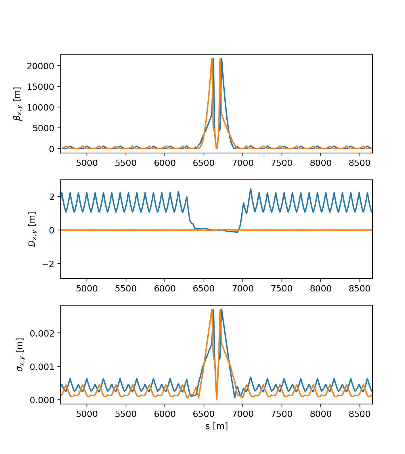
Beam sizes as obtained from twiss.
Particles normalized coordinates
The twiss table holds the information to convert particle physical coordinates
into normalized coordinates. This can be done with the method
get_normalized_coordinates as illustrated in the following example:
import numpy as np
import xtrack as xt

# Load a line
line = xt.load(
    '../../test_data/hllhc15_noerrors_nobb/line_and_particle.json')
line.set_particle_ref('proton', p0c=7e12)

# Generate some particles with known normalized coordinates
particles = line.build_particles(
    nemitt_x=2.5e-6, nemitt_y=1e-6,
    x_norm=[-1, 0, 0.5], y_norm=[0.3, -0.2, 0.2],
    px_norm=[0.1, 0.2, 0.3], py_norm=[0.5, 0.6, 0.8],
    zeta=[0, 0.1, -0.1], delta=[1e-4, 0., -1e-4])

# Inspect physical coordinates
tab = particles.get_table()
tab.show()
# prints
#
# Table: 3 rows, 17 cols
# particle_id s            x           px            y          py zeta   delta chi ...
#           0 0 -0.000253245  3.33271e-06  5.10063e-05 1.00661e-06    0  0.0001   1
#           1 0 -2.06127e-09  3.32087e-07 -3.42343e-05 5.59114e-08  0.1       0   1
#           2 0  0.000152331 -7.62878e-07  3.45785e-05  1.0462e-06 -0.1 -0.0001   1


# Compute twiss
tw = line.twiss()

# Use twiss to compute normalized coordinates
norm_coord = tw.get_normalized_coordinates(particles, nemitt_x=2.5e-6,
                                           nemitt_y=1e-6)

# Inspect normalized coordinates
norm_coord.show()
#
# Table: 3 rows, 8 cols
# particle_id at_element       x_norm px_norm y_norm py_norm   zeta_norm  pzeta_norm
#           0          0           -1     0.1    0.3     0.5 1.06651e-07  0.00313799
#           1          0 -1.59607e-20     0.2   -0.2     0.6  0.00318676 1.12046e-05
#           2          0          0.5     0.3    0.2     0.8  -0.0031868  -0.0031492

# Complete source: xtrack/examples/twiss/012_compute_norm_coordinates.py
Reverse reference frame
The reverse` flag, allows getting the output of the twiss in the counter-rotating reference system. When reverse is True, the ordering of the elements is reversed, the zero of the s` coordinate and of the phase advances is set at the new start, the sign of the coordinates s` and x` is inverted, while the sign of the coordinate y is unchanged. This is illustrated in the following example:
import xtrack as xt

# Load collider with two lines
collider = xt.load('../../test_data/hllhc15_thick/hllhc15_collider_thick.json')
collider.lhcb1.twiss_default.clear() # clear twiss default settings
collider.lhcb2.twiss_default.clear() # clear twiss default settings
collider['on_disp'] = 0 # disable dispersion correction

# Set a horizontal crossing angle between the two beams  in the interaction
# point ip1 and a vertical crossing angle in ip5
collider['on_x1hl'] = 10 # [urad]
collider['on_x5vl'] = 10 # [urad]
# Set a vertical separation between the two beams in the interaction point ip5
# and a horizontal separation in ip5
collider['on_sep1v'] = 0.5 # [mm]
collider['on_sep5h'] = 0.5 # [mm]

# Twiss the two lines (4d method since cavities are off)
tw1 = collider.lhcb1.twiss(method='4d')
tw2 = collider.lhcb2.twiss(method='4d')

tw1.reference_frame # is `proper`
tw2.reference_frame # is `proper`

# tw1 has a clokwise frame while tw2 has a counter-clockwise frame.
#
# name         s   mux   muy         x          y         px         py
# ip1          0     0     0 4.313e-09     0.0005  1.002e-05 -4.133e-09
# ip3       6665 15.95 15.45 2.392e-08 -2.209e-07  3.695e-10 -3.005e-09
# ip5  1.333e+04 30.93 29.99    0.0005  4.332e-09  1.918e-08      1e-05
# ip7  1.999e+04 46.35 44.59 2.138e-07 -1.785e-08 -2.132e-09 -3.078e-11

tw2.rows['ip[1,3,5,7]'].cols['s mux muy x y px py'].show(digits=4)
# prints:
#
# name         s   mux   muy          x          y         px         py
# ip7       6665 16.19 15.45 -5.941e-09   2.69e-07 -1.098e-10  2.428e-09
# ip5  1.333e+04 31.28 30.37     0.0005  5.997e-09 -4.562e-09  1.003e-05
# ip3  1.999e+04 46.46 44.81  -9.85e-08 -2.447e-08  3.218e-09 -9.711e-10
# ip1  2.666e+04 62.31 60.32 -2.278e-09    -0.0005     -1e-05   2.57e-08

# -- Reverse b2 twiss --
# The `reverse`` flag, allows getting the output of the twiss in the counter-rotating
# reference system. When `reverse` is True, the ordering of the elements is reversed,
# the zero of the s coordinate and fo the phase advances is set at  the new start,
# the sign of the coordinates s and x is inverted, while the sign of the coordinate
# y is unchanged. In symbols:
#
# s   -> L - s
# mux -> mux(L) - mux
# muy -> muy(L) - muy
# x   -> -x
# y   -> y
# px  -> px
# py  -> -py

tw2_r = collider.lhcb2.twiss(method='4d', reverse=True)
tw2_r.reference_frame # is `reverse`

tw2_r.rows['ip[1,3,5,7]'].cols['s mux muy x y px py'].show(digits=4)
# prints:
#
# name         s   mux   muy         x          y         px         py
# ip1  2.183e-11     0     0 2.278e-09    -0.0005     -1e-05  -2.57e-08
# ip3       6665 15.85 15.51  9.85e-08 -2.447e-08  3.218e-09  9.711e-10
# ip5  1.333e+04 31.03 29.95   -0.0005  5.997e-09 -4.562e-09 -1.003e-05
# ip7  1.999e+04 46.12 44.87 5.941e-09   2.69e-07 -1.098e-10 -2.428e-09

# In this way, for a collider, it is possible to plot the closed orbit and the
# twiss functions of the two beams in the same graph. For example:

import matplotlib.pyplot as plt
plt.close('all')
fig = plt.figure(1)

ax1 = fig.add_subplot(211)
ax1.plot(tw1.s, tw1.x * 1000, color='b', label='b1')
ax1.plot(tw2_r.s, tw2_r.x * 1000, color='r', label='b2')
ax1.set_ylabel('x [m]')
ax1.legend(loc='best')

ax2 = fig.add_subplot(212, sharex=ax1)
ax2.plot(tw1.s, tw1.y * 1000, color='b', label='b1')
ax2.plot(tw2_r.s, tw2_r.y * 1000, color='r', label='b1')
ax2.set_ylabel('y [mm]')
ax2.set_xlabel('s [mm]')

ax1.set_xlim(tw1['s', 'ip5'] - 300, tw1['s', 'ip5'] + 300)

ax1.axvline(x=tw1['s', 'ip5'], color='k', linestyle='--', alpha=0.5)
ax2.axvline(x=tw1['s', 'ip5'], color='k', linestyle='--', alpha=0.5)
plt.text(tw1['s', 'ip5'], -0.6, 'ip5', rotation=90, alpha=0.5,
         horizontalalignment='left', verticalalignment='top')

plt.show()

# Complete source: xtrack/examples/twiss/000e_twiss_reverse.py
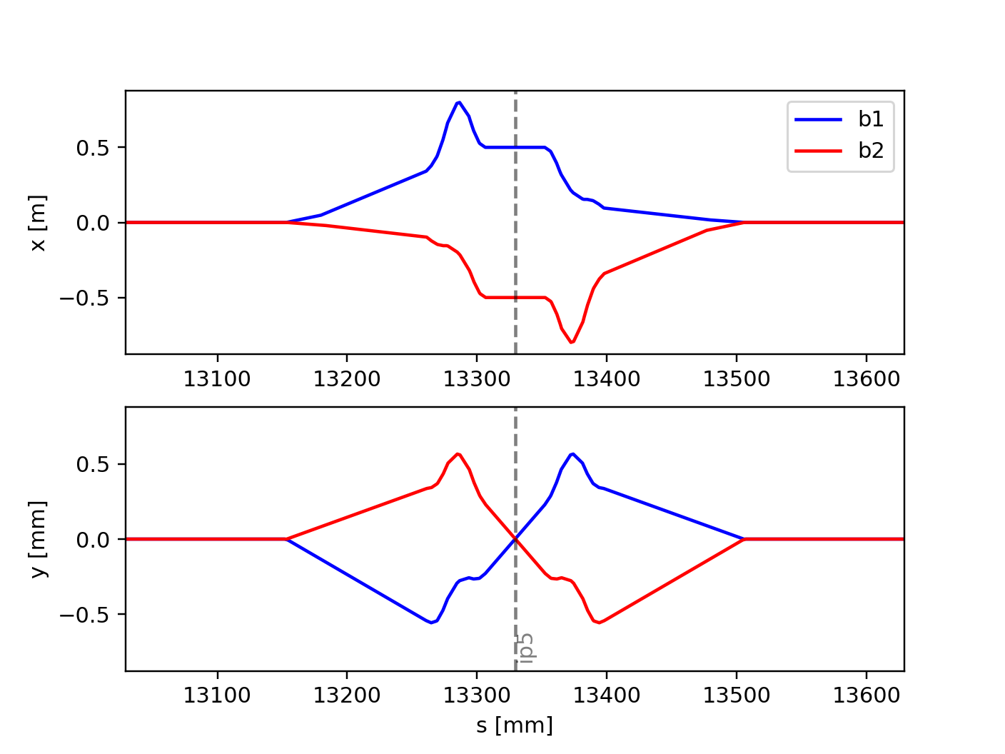
Closed Orbit of the two LHC beams in the same reference frame. This is
obtained setting reverse=True on the twiss of beam 2.
Twiss defaults
It is possible to change the default behavior of the twiss method for a given
line using line.twiss_defaults, which is a dictionary with the desired
default twiss arguments. This is illustrated in the following example:
import xtrack as xt

# Load a line
line = xt.load('../../test_data/hllhc15_noerrors_nobb/line_and_particle.json')
line.set_particle_ref('proton', energy0=7e12)

# Twiss (built-in defaults)
tw_a = line.twiss()
tw_a.method # is '6d'
tw_a.reference_frame # is 'proper'

# Inspect twiss defaults
line.twiss_default # is {}

# Set some twiss defaults
line.twiss_default['method'] = '4d'
line.twiss_default['reverse'] = True

# Twiss (defaults redefined)
tw_b = line.twiss()
tw_b.method # is '4d'
tw_b.reference_frame # is 'reverse'

# Inspect twiss defaults
line.twiss_default # is {'method': '4d', 'reverse': True}

# Reset twiss defaults
line.twiss_default.clear()

# Twiss (defaults reset)
tw_c = line.twiss()
tw_c.method # is '6d'
tw_c.reference_frame # is 'proper'

# Complete source: xtrack/examples/twiss/000f_twiss_default.py