Track

Tracking particles with Xsuite

The tracking of particles through a beam line can be simulated using the xtrack.Line.track() method of the xtrack.Line class. This is illustrated in the following example:

import numpy as np

import xobjects as xo
import xtrack as xt

## Generate a simple line
line = xt.Line(
    elements=[xt.Drift(length=2.),
              xt.Multipole(knl=[0, 0.5], ksl=[0,0]),
              xt.Drift(length=1.),
              xt.Multipole(knl=[0, -0.5], ksl=[0,0])],
    element_names=['drift_0', 'quad_0', 'drift_1', 'quad_1'])

## Attach a reference particle to the line (optional)
## (defines the reference mass, charge and energy)
line.particle_ref = xt.Particles(p0c=6500e9, #eV
                                 q0=1, mass0=xt.PROTON_MASS_EV)

## Choose a context
context = xo.ContextCpu()         # For CPU
# context = xo.ContextCupy()      # For CUDA GPUs
# context = xo.ContextPyopencl()  # For OpenCL GPUs

## Transfer lattice on context and compile tracking code
line.build_tracker(_context=context)

## Build particle object on context
n_part = 20
particles = line.build_particles(
                        x=np.random.uniform(-1e-3, 1e-3, n_part),
                        px=np.random.uniform(-1e-5, 1e-5, n_part),
                        y=np.random.uniform(-2e-3, 2e-3, n_part),
                        py=np.random.uniform(-3e-5, 3e-5, n_part),
                        zeta=np.random.uniform(-1e-2, 1e-2, n_part),
                        delta=np.random.uniform(-1e-4, 1e-4, n_part))
# Reference mass, charge, energy are taken from the reference particle.
# Particles are allocated on the context chosen for the line.

## Track (no saving of turn-by-turn data)
n_turns = 100
line.track(particles, num_turns=n_turns)

particles.state # > 0 for particles still alive
particles.at_turn # turn number (for lost particles, it is the turn of loss)
particles.x # x position after tracking
particles.px # x momentum after tracking
# etc...

## Track (saving turn-by-turn data)
particles = line.build_particles( # fresh particles
                        x=np.random.uniform(-1e-3, 1e-3, n_part),
                        px=np.random.uniform(-1e-5, 1e-5, n_part),
                        y=np.random.uniform(-2e-3, 2e-3, n_part),
                        py=np.random.uniform(-3e-5, 3e-5, n_part),
                        zeta=np.random.uniform(-1e-2, 1e-2, n_part),
                        delta=np.random.uniform(-1e-4, 1e-4, n_part))
n_turns = 100
line.track(particles, num_turns=n_turns,
              turn_by_turn_monitor=True)

## Turn-by-turn data is available at:
line.record_last_track.x
line.record_last_track.px
# etc...

# Complete source: xtrack/examples/tracker/000_track.py

Dynamic aperture

The following example illustrate how to use Xsuite to study the Dynamic Aperture of a ring.

import numpy as np

import xtrack as xt
import xpart as xp
import xobjects as xo

line = xt.Line.from_json(
    '../../test_data/hllhc14_no_errors_with_coupling_knobs/line_b1.json')
line.build_tracker()

# Switch on LHC octupole circuits to have a smaller dynamic aperture
for arc in ['12', '23', '34', '45', '56', '67', '78', '81']:
    line.vars[f'kod.a{arc}b1'] = 2.0
    line.vars[f'kof.a{arc}b1'] = 2.0

# Generate normalized particle coordinates on a polar grid
n_r = 50
n_theta = 60
x_normalized, y_normalized, r_xy, theta_xy = xp.generate_2D_polar_grid(
    r_range=(0, 40.), # beam sigmas
    theta_range=(0, np.pi/2),
    nr=n_r, ntheta=n_theta)

# Set initial momentum deviation
delta_init = 0 # In case off-momentum DA is needed

# Match particles to the machine optics and orbit
particles = line.build_particles(
    x_norm=x_normalized, px_norm=0,
    y_norm=y_normalized, py_norm=0,
    nemitt_x=3e-6, nemitt_y=3e-6, # normalized emittances
    delta=delta_init)

# # Optional: activate multi-core CPU parallelization
# line.discard_tracker()
# line.build_tracker(_context=xo.ContextCpu(omp_num_threads='auto'))

# Track
line.track(particles, num_turns=200, time=True)

print(f'Tracked in {line.time_last_track} seconds')

# Sort particles to get the initial order
# (during tracking lost particles are moved to the end)
particles.sort(interleave_lost_particles=True)

# Plot result using scatter or pcolormesh
import matplotlib.pyplot as plt
plt.close('all')
plt.figure(1)
plt.scatter(x_normalized, y_normalized, c=particles.at_turn)
plt.xlabel(r'$A_x [\sigma]$')
plt.ylabel(r'$A_y [\sigma]$')
cb = plt.colorbar()
cb.set_label('Lost at turn')

plt.figure(2)
plt.pcolormesh(
    x_normalized.reshape(n_r, n_theta), y_normalized.reshape(n_r, n_theta),
    particles.at_turn.reshape(n_r, n_theta), shading='gouraud')
plt.xlabel(r'$A_x [\sigma]$')
plt.ylabel(r'$A_y [\sigma]$')
ax = plt.colorbar()
ax.set_label('Lost at turn')

plt.show()

# Complete source: xtrack/examples/dynamic_aperture/000_tracking_for_da.py

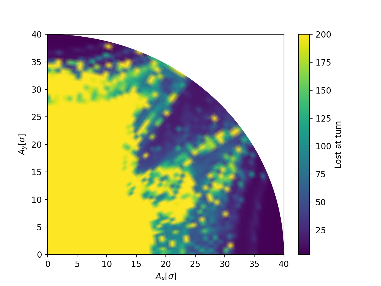
On-momentum dynamic aperture for the LHC lattice with octupoles active.

Monitors

See also: xtrack.ParticlesMonitor, xtrack.LastTurnsMonitor, xtrack.BeamPositionMonitor, xtrack.BeamProfileMonitor, xtrack.BeamSizeMonitor.

The easy way

When starting a tracking simulation with the Xtrack Line object, the easiest way of logging the coordinates of all particles for all turns is to enable the default turn-by-turn monitor, as illustrated by the following example. Note: this mode requires that particles.at_turn is 0 for all particles at the beginning of the simulation.

import json

import xtrack as xt
import xpart as xp
import xobjects as xo

context = xo.ContextCpu()

with open('../../test_data/hllhc15_noerrors_nobb/line_and_particle.json') as f:
    dct = json.load(f)
line = xt.Line.from_dict(dct['line'])
line.particle_ref = xt.Particles.from_dict(dct['particle'])

line.build_tracker()

num_particles = 50
particles = xp.generate_matched_gaussian_bunch(line=line,
                                               num_particles=num_particles,
                                               nemitt_x=2.5e-6,
                                               nemitt_y=2.5e-6,
                                               sigma_z=9e-2)

num_turns = 30
line.track(particles, num_turns=num_turns,
              turn_by_turn_monitor=True # <--
             )
# line.record_last_track contains the measured data. For example,
# line.record_last_track.x contains the x coordinate for all particles
# and all turns, e.g. line.record_last_track.x[3, 5] for the particle
# having particle_id = 3 and for the turn number 5.

# Monitor objects can be dumped to a dictionary and loaded back
mon = line.record_last_track
dct = mon.to_dict()
mon2 = xt.ParticlesMonitor.from_dict(dct)

# Complete source: xtrack/examples/monitor/000_example_quick_monitor.py

Custom monitors

In order to customize the monitor’s behaviour, a custom monitor object can be built and passed to the Line.track function.

Particles coordinates can be recorded only in a selected range of turns by specifying start_at_turn and stop_at_turn. The monitoring can also be limited to a selected range of particles IDs, by using the argument particle_id_range of the ParticlesMonitor class to provide a tuple defining the range to be recorded. In that case the num_particles input of the monitor is omitted.

The example above is changed as follows:

...

monitor = xt.ParticlesMonitor(_context=context,
    particle_id_range=(5, 42),
    start_at_turn=5, # <-- first turn to monitor (including)
    stop_at_turn=15, # <-- last turn to monitor (excluding)
)

line.track(particles, num_turns=num_turns,
           turn_by_turn_monitor=monitor, # <-- pass the monitor here
)

Now, line.record_last_track.x[3, 5] gives the x coordinates for the particle 3 (which has the id 8) and the recorded turn 5 (which is turn number 10) The particle ids that are recorded can be inspected in line.record_last_track.particle_id and the turn indeces in line.record_last_track.at_turn.

Multi-frame particles monitor

The particles monitor can also record periodically spaced intervals of turns (frames) This feature can be activated by providing the arguments n_repetitions and repetition_period when creating the monitor. In the following example, we record turns in range 5 to 10 (first frame), range 25 to 30 (second frame) and range 45 to 50 (third frame). Note that each frame consists of 5 turns since stop_at_turn is excluding.

monitor = xt.ParticlesMonitor(_context=context,
    num_particles=num_particles,
    start_at_turn=5,
    stop_at_turn=10,
    n_repetitions=3,      # <--
    repetition_period=20, # <--
)

Now, the measured data are 3D array with the first index being the frame number. For example, line.record_last_track.x[0, :, :] contains the recorded x position for the first frame (turns 5, 6, 7, 8 and 9) and line.record_last_track.x[-1, :, 0] refers to the last frame and the first turn within, which is turn number turn 25. As before, the turn numbers recorded can be inspected with line.record_last_track.at_turn.

Particles monitor as beam elements

Particles monitors can be used as regular beam element to record the particle coordinates at specific locations in the beam line. For this purpose they can be inserted in the line, as illustrated in the following example.

import json

import xtrack as xt
import xpart as xp
import xobjects as xo

context = xo.ContextCpu()

with open('../../test_data/hllhc15_noerrors_nobb/line_and_particle.json') as f:
    dct = json.load(f)
line = xt.Line.from_dict(dct['line'])
line.particle_ref = xt.Particles.from_dict(dct['particle'])

num_particles = 50
monitor_ip5 = xt.ParticlesMonitor(start_at_turn=5, stop_at_turn=15,
                                    num_particles=num_particles)
monitor_ip8 = xt.ParticlesMonitor(start_at_turn=5, stop_at_turn=15,
                                    num_particles=num_particles)
line.insert_element(index='ip5', element=monitor_ip5, name='mymon5')
line.insert_element(index='ip8', element=monitor_ip8, name='mymon8')

line.build_tracker()

particles = xp.generate_matched_gaussian_bunch(line=line,
                                               num_particles=num_particles,
                                               nemitt_x=2.5e-6,
                                               nemitt_y=2.5e-6,
                                               sigma_z=9e-2)

num_turns = 30
monitor = xt.ParticlesMonitor(_context=context,
                              start_at_turn=5, stop_at_turn=15,
                              num_particles=num_particles)
line.track(particles, num_turns=num_turns)

# monitor_ip5 contains the data recorded in before the element 'ip5', while
# monitor_ip8 contains the data recorded in before the element 'ip8'
# The element index at which the recording is made can be inspected in
# monitor_ip5.at_element.

# Complete source: xtrack/examples/monitor/003_monitors_as_beam_elements.py

As all Xtrack elements, the Particles Monitor has a track method and can be used in stand-alone mode as illustrated in the following example.

# line.track(particles, num_turns=num_turns)
for iturn in range(num_turns):
    monitor.track(particles)
    line.track(particles)

Last turns monitor

The xtrack.LastTurnsMonitor records particle data in the last turns before respective particle loss (or the end of tracking).

The idea is to use a rolling buffer instead of saving all the turns. This saves a lot of memory resources when the interest lies only in the last few turns. For each particle, the recorded data will cover up to n_last_turns*every_n_turns turns before it is lost (or the tracking ends).

monitor = LastTurnsMonitor(
    particle_id_range=(0, 5),
    n_last_turns=5,            # amount of turns to store
    every_n_turns=3,           # only consider turns which are a multiples of this
)

... # track

monitor.at_turn[:,-1]  # turn number of each particle before it is lost (last turn alive)
monitor.x[3,-2]        # x coordinate of particle 3 in one but last turn (-2)

The monitor provides the following data as 2D array of shape (num_particles, n_last_turns), where the first index corresponds to the particle in particle_id_range and the second index corresponds to the turn (or every_n_turns) before the respective particle is lost: particle_id, at_turn, x, px, y, py, delta, zeta

Beam position monitor

The xtrack.BeamPositionMonitor records transverse beam positions, i.e. it stores the x and y centroid positions of particles. This can be useful for tune or beam-transfer-function diagnostics as well as transverse schottky spectra.

The monitor allows for arbitrary sampling frequencies and can thus not only be used for bunch positions, but also coasting beam positions. Higher sampling frequencies give access to transverse beam oscillations at higher harmonics, which is especially useful for schottky diagnostics. Internally, the particle arrival time is used when determining the record index. For coasting beams this ensures, that the centroid is computed considering all particles which arrive at the monitor at the same time (as in a real-world measurement device), even if some particles might have made more or less turns than the synchronous particle due to a non-negligible momentum deviation.

\[i = f_{samp} \times \left(\frac{n-n_0}{f_{rev}} - \frac{\zeta}{\beta_0 c_0}\right)\]

where \(f_{samp}\) is the sampling frequency, \(f_{rev}\) is the revolution frequency, \(n\) is the current turn number and \(n_0\) is the first turn recorded, \(\zeta=(s-\beta_0\cdot c_0\cdot t)\) is the longitudinal zeta coordinate of the particle, \(\beta_0\) is the relativistic beta factor of the particle and \(c_0\) is the speed of light. For non-circular lines \(n\) is always zero and \(f_{rev}\) can be omitted.

Note that the index is rounded, i.e. the result array represents data of particles equally distributed around the reference particle, which is useful for bunched beams. For example, if the sampling frequency is twice the revolution frequency, the first item contains data from particles in the range zeta/circumference = -0.25 .. 0.25, the second item in the range 0.25 .. 0.75 and so on.

monitor = xt.BeamPositionMonitor(
    #particle_id_range=(5, 42),        # optional, defaults to all particles if not given
    start_at_turn=5, stop_at_turn=10,  # turn refers to the synchronous particle (at zeta=0)
    frev=1e6,                          # revolution frequency (only for circular lines)
    sampling_frequency=2e6,            # sampling frequency
)

... # track

print(monitor.count)   # waveform of number of particles (intensity)
print(monitor.x_mean)  # waveform of horizontal centroid positions (alias monitor.x_cen)
print(monitor.y_mean)  # waveform of vertical centroid positions (alias monitor.y_cen)

The result arrays can be understood as waveforms recorded at the specified sampling frequency. In the special case where sampling frequency was set to the same value as the revolution frequency, the indices are identical to the recorded turn numbers (of the synchronous particle).

Beam size monitor

The xtrack.BeamSizeMonitor records transverse beam sizes, i.e. it stores the standard deviation of the particles x and y positions.

Like the Beam position monitor also the beam size monitor is based on particle arrival time and an arbitrary sampling frequency.

monitor = xt.BeamSizeMonitor(
    #particle_id_range=(5, 42),        # optional, defaults to all particles if not given
    start_at_turn=5, stop_at_turn=10,  # turn refers to the synchronous particle (at zeta=0)
    frev=1e6,                          # revolution frequency (only for circular lines)
    sampling_frequency=2e6,            # sampling frequency
)

... # track

print(monitor.count)   # waveform of number of particles (intensity)
print(monitor.x_mean)  # waveform of horizontal centroid positions
print(monitor.y_std)   # waveform of vertical position standard deviation (i.e. beam size)
print(monitor.x_var)   # waveform of horizontal position variances

Beam profile monitor

The xtrack.BeamProfileMonitor records transverse beam profiles, i.e. it stores the number of particles on a defined raster (like a histogram).

Like the Beam position monitor also the beam profile monitor is based on particle arrival time and an arbitrary sampling frequency.

monitor = xt.BeamProfileMonitor(
    #particle_id_range=(5, 42),        # optional, defaults to all particles if not given
    start_at_turn=5, stop_at_turn=10,  # turn refers to the synchronous particle (at zeta=0)
    frev=1e6,                          # revolution frequency (only for circular lines)
    sampling_frequency=2e6,            # sampling frequency
    n=100,                             # number of bins in the profile (can also specify nx and ny separately)
    x_range=(-4,2),                    # save horizontal profile extending from -4 to 2
    y_range=5,                         # shorthand for (-2.5, 2.5)
)

... # track

print(monitor.x_edges)      # the bin edges
print(monitor.x_grid)       # the bin midpoints
print(monitor.x_intensity)  # the actual profile (particle count per bin)

The recorded profiles are 2D arrays of shape (sample_size, n) where sample_size = round(( stop_at_turn - start_at_turn ) * sampling_frequency / frev). I.e. monitor.x_intensity[0,:] is the first recorded profile and monitor.x_intensity[-1,:] the last.

Start/stop tracking at specific elements

It is possible to start and/or stop the tracking at specific elements of the beam line. This is illustrated in the following example:

import xtrack as xt

### Behavior:

# For num_turns = 1 (default):
#  - line.track(particles, ele_start=3, ele_stop=5) tracks once from element 3 to
#    element 5 e. particles.at_turn is not incremented as the particles never pass through
#    the end of the beam line.
#  - line.track(particles, ele_start=7, ele_stop=3) tracks once from element 5 to
#    the end of the beamline and then from element 0 to element 3 excluded.
#    particles.at_turn is incremented to one as the particles pass once
#    the end of the beam line.

# When indicating num_turns = N with N > 1, additional (N-1) full turns are added to logic
# above. Therefore:
# - if ele_stop < ele_start: stops at element ele_stop when particles.at_turn = N - 1
# - if ele_stop >= ele_start: stops at element ele_stop when particles.at_turn = N

elements = [xt.Drift(length=1.) for _ in range(10)]
line=xt.Line(elements=elements)
line.build_tracker()
line.reset_s_at_end_turn = False

# Standard mode
p = xt.Particles(x=[1e-3, 2e-3, 3e-3], p0c=7e12)
line.track(p, num_turns=4)
p.at_turn # is [4, 4, 4]

# ele_start > 0
p = xt.Particles(x=[1e-3, 2e-3, 3e-3], p0c=7e12, s=4., at_element=2)
line.track(p, num_turns=3, ele_start=2)
p.at_turn # is [3, 3, 3]

# 0 <= ele_start < ele_stop
p = xt.Particles(x=[1e-3, 2e-3, 3e-3], p0c=7e12, s=5 * 2., at_element=5)
line.track(p, num_turns=4, ele_start=5, ele_stop=8)
p.at_turn # is [3, 3, 3]

# 0 <= ele_start < ele_stop -- num_turns = 1
p = xt.Particles(x=[1e-3, 2e-3, 3e-3], p0c=7e12, s=5 * 2., at_element=5)
line.track(p, num_turns=1, ele_start=5, ele_stop=2)
p.at_turn # is [1, 1, 1]

# 0 <= ele_start < ele_stop -- num_turns > 1
p = xt.Particles(x=[1e-3, 2e-3, 3e-3], p0c=7e12, s=5 * 2., at_element=5)
line.track(p, num_turns=4, ele_start=5, ele_stop=2)
p.at_turn # is [4, 4, 4]

# Use ele_start and num_turns
p = xt.Particles(x=[1e-3, 2e-3, 3e-3], p0c=7e12, s=5 * 2., at_element=5)
line.track(p, ele_start=5, num_elements=7)
p.at_turn # is [1, 1, 1]

# Complete source: xtrack/examples/tracker/001_tracker_start_stop.py

Backtracking

It is possible to track particles backwards through a beam line, provided that all elements included in the line support backtracking. The following example illustrates how backtrack for a full turn or between specified elements:

import xtrack as xt

line = xt.Line.from_json(
    '../../test_data/hllhc15_noerrors_nobb/line_w_knobs_and_particle.json')
line.build_tracker()

p = xt.Particles(
    p0c=7000e9, x=1e-4, px=1e-6, y=2e-4, py=3e-6, zeta=0.01, delta=1e-4)
p.get_table().show(digits=3)
# prints:
#
# particle_id s      x    px      y    py zeta  delta chi ...
#           0 0 0.0001 1e-06 0.0002 3e-06 0.01 0.0001   1

# Track one turn
line.track(p)
p.get_table().show()
# prints:
#
# particle_id s        x        px        y        py    zeta  delta chi ...
#           0 0 0.000324 -1.07e-05 1.21e-05 -1.42e-06 0.00909 0.0001   1

# Track back one turn
line.track(p, backtrack=True)
# The particle is back to the initial coordinates
p.get_table().show(digits=3)
# prints:
#
# particle_id s      x    px      y    py zeta  delta chi ...
#           0 0 0.0001 1e-06 0.0002 3e-06 0.01 0.0001   1

# It is also possible to backtrack with a specified start/stop elements

# Track three elements
line.track(p, ele_start=0, ele_stop=3)
p.get_table().cols['x px y py zeta delta at_element'].show()
# prints:
#
# particle_id           x    px           y    py zeta  delta at_element
#           0 0.000121028 1e-06 0.000263084 3e-06 0.01 0.0001          3

# Track back three elements
line.track(p, ele_start=0, ele_stop=3, backtrack=True)
p.get_table().cols['x px y py zeta delta at_element'].show()
# prints:
#
# particle_id      x    px      y    py zeta  delta at_element
#           0 0.0001 1e-06 0.0002 3e-06 0.01 0.0001          0

# Complete source: xtrack/examples/tracker/002_backtrack.py

Freeze longitudinal coordinates

In certain studies, it is convenient to track particles updating only the transverse coordinates, while keeping the longitudinal coordinates fixed (frozen). Xsuite offers the possibility to freeze the longitudinal coordinates within a single method or changing the state of the Line, as illustrated in the following sections.

Freezing longitudinal when calling methods

The Line.twiss and Line.track can work with frozen longitudinal coordinates. This is done by setting the freeze_longitudinal argument to True, as shown in the following example:

import json

import xtrack as xt

# import a line and add reference particle
line = xt.Line.from_json(
    '../../test_data/hllhc15_noerrors_nobb/line_w_knobs_and_particle.json')
line.particle_ref = xt.Particles(mass0=xt.PROTON_MASS_EV, p0c=7e12)

# Build the tracker
line.build_tracker()

# Track some particles with frozen longitudinal coordinates
particles = line.build_particles(delta=1e-3, x=[-1e-3, 0, 1e-3])
line.track(particles, num_turns=10, freeze_longitudinal=True)
print(particles.delta) # gives [0.001 0.001 0.001], same as initial value

# Twiss with frozen longitudinal coordinates (needs to be 4d)
twiss = line.twiss(method='4d', freeze_longitudinal=True)
print(twiss.slip_factor) # gives 0 (no longitudinal motion)

# Track some particles with unfrozen longitudinal coordinates
particles = line.build_particles(delta=1e-3, x=[-1e-3, 0, 1e-3])
line.track(particles, num_turns=10)
print(particles.delta) # gives [0.00099218, ...], different from initial value

# Twiss with unfrozen longitudinal coordinates (can be 6d)
twiss = line.twiss(method='6d')
print(twiss.slip_factor) # gives 0.00032151, from longitudinal motion

# Complete source: xtrack/examples/freeze_longitudinal/002_freeze_individual_methods.py

Freezing longitudinal coordinates within a with block

A context manager is also available to freeze the longitudinal coordinates within a with block. The normal tracking mode, updating the longitudinal coordinates, is automatically restored when exiting the with block, as it is illustrated in the following example:

import json

import xtrack as xt

# import a line and add reference particle
# import a line and add reference particle
line = xt.Line.from_json(
    '../../test_data/hllhc15_noerrors_nobb/line_w_knobs_and_particle.json')
line.particle_ref = xt.Particles(mass0=xt.PROTON_MASS_EV, p0c=7e12)

# Build the tracker
line.build_tracker()

# Perform a set of operations with frozen longitudinal coordinates
with xt.freeze_longitudinal(line):
    # Track some particles with frozen longitudinal coordinates
    particles = line.build_particles(delta=1e-3, x=[-1e-3, 0, 1e-3])
    line.track(particles, num_turns=10)
    print(particles.delta) # gives [0.001 0.001 0.001], same as initial value

    # Twiss with frozen longitudinal coordinates (needs to be 4d)
    twiss = line.twiss(method='4d')
    print(twiss.slip_factor) # gives 0 (no longitudinal motion)

# 6d tracking is automatically restored when the with block is exited

# Track some particles with unfrozen longitudinal coordinates
particles = line.build_particles(delta=1e-3, x=[-1e-3, 0, 1e-3])
line.track(particles, num_turns=10)
print(particles.delta) # gives [0.00099218, ...], different from initial value

# Twiss with unfrozen longitudinal coordinates (can be 6d)
twiss = line.twiss(method='6d')
print(twiss.slip_factor) # gives 0.00032151, from longitudinal motion

# Complete source: xtrack/examples/freeze_longitudinal/001_freeze_context_manager.py

Freezing longitudinal coordinates with Line method

The xtrack.Line class provides a method called freeze_longitudinal() to explicitly freeze the longitudinal coordinates. The normal tracking mode, updating the longitudinal coordinates, can be restored by calling freeze_longitudinal(False). This is illustrated in the following example:

import xtrack as xt

# import a line and add reference particle
line = xt.Line.from_json(
    '../../test_data/hllhc15_noerrors_nobb/line_w_knobs_and_particle.json')
line.particle_ref = xt.Particles(mass0=xt.PROTON_MASS_EV, p0c=7e12)

# Build the tracker
line.build_tracker()

# Freeze longitudinal coordinates
line.freeze_longitudinal()

# Track some particles with frozen longitudinal coordinates
particles = line.build_particles(delta=1e-3, x=[-1e-3, 0, 1e-3])
line.track(particles, num_turns=10)
print(particles.delta) # gives [0.001 0.001 0.001], same as initial value

# Twiss with frozen longitudinal coordinates (needs to be 4d)
twiss = line.twiss(method='4d')
print(twiss.slip_factor) # gives 0 (no longitudinal motion)

# Unfreeze longitudinal coordinates
line.freeze_longitudinal(False)

# Track some particles with unfrozen longitudinal coordinates
particles = line.build_particles(delta=1e-3, x=[-1e-3, 0, 1e-3])
line.track(particles, num_turns=10)
print(particles.delta) # gives [0.00099218, ...], different from initial value

# Twiss with unfrozen longitudinal coordinates (can be 6d)
twiss = line.twiss(method='6d')
print(twiss.slip_factor) # gives 0.00032151, from longitudinal motion

# Complete source: xtrack/examples/freeze_longitudinal/000_freeze_unfreeze_explicit.py

Time-dependent line properties

Time dependent knobs

To simulate the effect of time-changing properties of the beam-line it is possible to control any lattice element attribute with a time-dependent function. For this purpose, the variable t_turn_s provides the time in seconds since the start of the simulation and is updated automatically during tracking. The simulation of an orbit bump driven by a sinusoidal function is shown in the following example.

import numpy as np
import matplotlib.pyplot as plt

import xtrack as xt

# Define elements
pi = np.pi
lbend = 3
elements = {
    # Three dipoles to make a closed orbit bump
    'd0.1':  xt.Drift(length=0.05),
    'bumper_0':  xt.Bend(length=0.05, k0=0, h=0),
    'd0.2':  xt.Drift(length=0.3),
    'bumper_1':  xt.Bend(length=0.05, k0=0, h=0),
    'd0.3':  xt.Drift(length=0.3),
    'bumper_2':  xt.Bend(length=0.05, k0=0, h=0),
    'd0.4':  xt.Drift(length=0.2),

    # Simple ring with two FODO cells
    'mqf.1': xt.Quadrupole(length=0.3, k1=0.1),
    'd1.1':  xt.Drift(length=1),
    'mb1.1': xt.Bend(length=lbend, k0=pi / 2 / lbend, h=pi / 2 / lbend),
    'd2.1':  xt.Drift(length=1),
    'mqd.1': xt.Quadrupole(length=0.3, k1=-0.7),
    'd3.1':  xt.Drift(length=1),
    'mb2.1': xt.Bend(length=lbend, k0=pi / 2 / lbend, h=pi / 2 / lbend),
    'd3.4':  xt.Drift(length=1),
    'mqf.2': xt.Quadrupole(length=0.3, k1=0.1),
    'd1.2':  xt.Drift(length=1),
    'mb1.2': xt.Bend(length=lbend, k0=pi / 2 / lbend, h=pi / 2 / lbend),
    'd2.2':  xt.Drift(length=1),
    'mqd.2': xt.Quadrupole(length=0.3, k1=-0.7),
    'd3.2':  xt.Drift(length=1),
    'mb2.2': xt.Bend(length=lbend, k0=pi / 2 / lbend, h=pi / 2 / lbend),

}

# Build the ring
line = xt.Line(elements=elements, element_names=list(elements.keys()))
kin_energy_0 = 50e6 # 50 MeV
line.particle_ref = xt.Particles(energy0=kin_energy_0 + xt.PROTON_MASS_EV, # total energy
                                 mass0=xt.PROTON_MASS_EV)

# Twiss
tw = line.twiss(method='4d')

# Power the correctors to make a closed orbit bump
line.vars['bumper_strength'] = 0.
line.element_refs['bumper_0'].k0 = -line.vars['bumper_strength']
line.element_refs['bumper_1'].k0 = 2 * line.vars['bumper_strength']
line.element_refs['bumper_2'].k0 = -line.vars['bumper_strength']

# Drive the correctors with a sinusoidal function
T_sin = 100e-6
sin = line.functions.sin
line.vars['bumper_strength'] = (0.1 * sin(2 * np.pi / T_sin * line.vars['t_turn_s']))


# --- Probe behavior with twiss at different t_turn_s ---

t_test = np.linspace(0, 100e-6, 15)
tw_list = []
bumper_0_list = []
for tt in t_test:
    line.vars['t_turn_s'] = tt
    bumper_0_list.append(line.element_refs['bumper_0'].k0) # Inspect bumper
    tw_list.append(line.twiss(method='4d')) # Twiss

# Plot
plt.close('all')
plt.figure(1, figsize=(6.4*1.2, 4.8*0.85))
ax1 = plt.subplot(1, 2, 1, xlabel='Time [us]', ylabel='x at bump center [mm]')
ax2 = plt.subplot(1, 2, 2, xlabel='s [m]', ylabel='x [mm]')

colors = plt.cm.jet(np.linspace(0, 1, len(t_test)))

for ii, tt in enumerate(t_test):
    tw_tt = tw_list[ii]
    ax1.plot(tt * 1e6, tw_tt['x', 'bumper_1'] * 1e3, 'o', color=colors[ii])
    ax2.plot(tw_tt.s, tw_tt.x * 1e3, color=colors[ii], label=f'{tt * 1e6:.1f} us')

ax2.set_xlim(0, tw_tt['s', 'bumper_2'] + 1)
plt.subplots_adjust(left=.1, right=.97, top=.92, wspace=.27)
ax2.legend()


# --- Track particles with time-dependent bumpers ---

num_particles = 100
num_turns = 1000

# Install monitor in the middle of the bump
monitor = xt.ParticlesMonitor(num_particles=num_particles,
                              start_at_turn=0,
                              stop_at_turn =num_turns)
line.discard_tracker()
line.insert_element('monitor', monitor, index='bumper_1')
line.build_tracker()

# Generate particles
particles = line.build_particles(
                        x=np.random.uniform(-0.1e-3, 0.1e-3, num_particles),
                        px=np.random.uniform(-0.1e-3, 0.1e-3, num_particles))

# Enable time-dependent variables
line.enable_time_dependent_vars = True

# Track
line.track(particles, num_turns=num_turns, with_progress=True)

# Plot
plt.figure(2, figsize=(6.4*0.8, 4.8*0.8))
plt.plot(1e6 * monitor.at_turn.T * tw.T_rev0, 1e3 * monitor.x.T,
         lw=1, color='r', alpha=0.05)
plt.plot(1e6 * monitor.at_turn[0, :] * tw.T_rev0, 1e3 * monitor.x.mean(axis=0),
         lw=2, color='k')
plt.xlabel('Time [us]')
plt.ylabel('x [mm]')
plt.show()

# Complete source: xtrack/examples/toy_ring/006a_dynamic_bump_sin.py

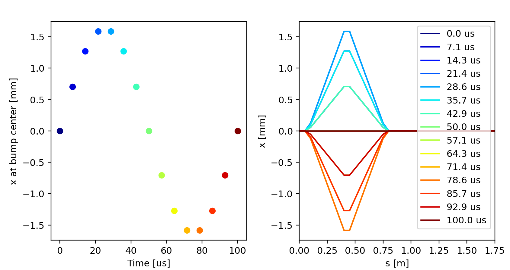
Orbit bump behavior as obained from the twiss for different settings of t_turn_s.

Beam position at the bump center during the tracking simulation. The red lines indicate the position of individual particles, the black line is their average position.

# Control the bumpers with a piece-wise linear function of time
# (outside the defined time interval, first and last point are held constant)
line.functions['my_fun'] = xt.FunctionPieceWiseLinear(
    x=np.array([10,    40,     70,   100]) * 1e-6, # time in s
    y=np.array([0,    0.5,    0.5,   1.0])        # value
)
line.vars['bumper_strength'] = 0.1 * line.functions['my_fun'](line.vars['t_turn_s'])

# Complete source: xtrack/examples/toy_ring/006b_dynamic_bump_piece_wise_linear.py

Instead of built-in functions, it is also possible to use piece-wise linear functions defined by the user. For example, the function in the figure below can be obtained with the following code:

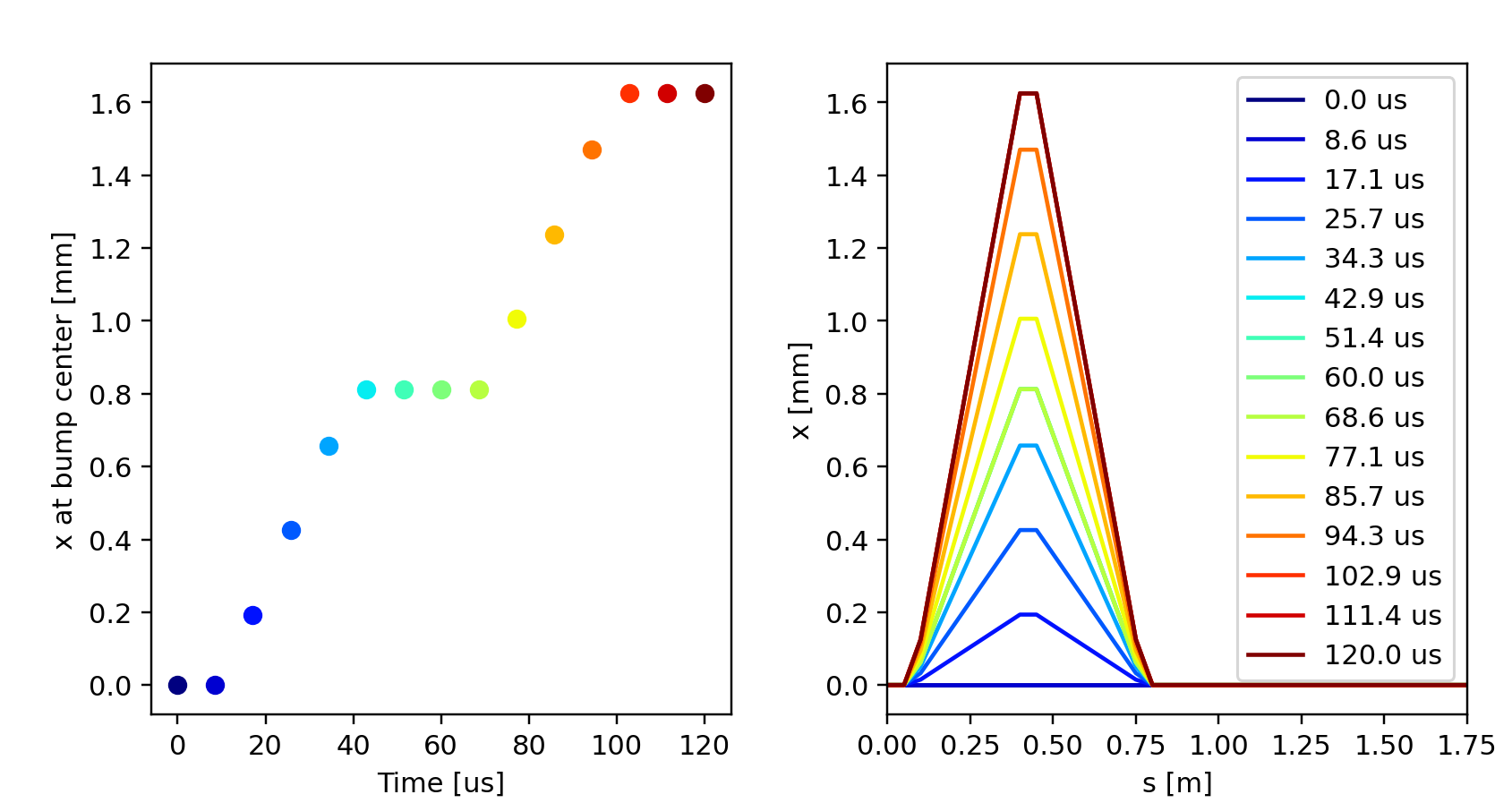
Orbit bump behavior as obained from the twiss for different settings of t_turn_s.

Beam position at the bump center during the tracking simulation. The red lines indicate the position of individual particles, the black line is their average position.

It is also possible to combine piece-wise linear functions with built-in functions in the same expression. For example, the following code can be used to generate a modulated sinusoidal function:

# Control the bumpers with a modulated sinusoidal function of time
line.functions['pulse'] = xt.FunctionPieceWiseLinear(
    x=np.array([10, 50, 150, 190]) * 1e-6, # s
    y=np.array([0,   1,   1,   0])         # knob value
)

T_sin = 10e-6
sin = line.functions.sin
line.vars['bumper_strength'] = (0.1 * line.functions['pulse'](line.vars['t_turn_s'])
                                * sin(2 * np.pi / T_sin * line.vars['t_turn_s']))

# Complete source: xtrack/examples/toy_ring/006c_dynamic_bump_sin_env.py

Beam position at the bump center during the tracking simulation. The red lines indicate the position of individual particles, the black line is their average position.

Multisetters

When the number of beam elements to be changed is very large, this can introduce a significant overhead on the simulation time. For these cases it is possible to use the xtrack.MultiSetter class, to perform the changes in a more efficient way, bypassing the expressions and acting directly on the element properties. Furthermore, the MultiSetter stores the memory addresses of the quantities to be changed and performs the changes with a single compiled kernel, using multithreading when allowed by the context.

The following example shows how to use the MultiSetter to apply a sinusoidal ripple to the strength of several quadropoles of a synchrotron.

See also: xtrack.MultiSetter

import numpy as np
from cpymad.madx import Madx

import xobjects as xo
import xtrack as xt
import xpart as xp

# Choose a context
ctx = xo.ContextCpu()

# Import SPS lattice and build a tracker
mad = Madx()
seq_name = 'sps'
mad.call('../../test_data/sps_w_spacecharge/sps_thin.seq')
mad.use(seq_name)
madtw = mad.twiss()

line = xt.Line.from_madx_sequence(mad.sequence[seq_name])
line.particle_ref = xt.Particles(p0c=400e9, mass0=xt.PROTON_MASS_EV)
line.build_tracker(_context=ctx)

# Switch on RF and twiss
line['acta.31637'].voltage = 7e6
line['acta.31637'].lag = 180.
twxt = line.twiss()

# Get revolution period
T_rev = twxt['T_rev0']

# Extract list of elements to trim (all focusing quads)
tt = line.get_table()
elements_to_trim = tt.rows[tt.element_type == 'Multipole'].rows['qf.*'].name
# => contains ['qf.52010', 'qf.52210', 'qf.52410', 'qf.52610', 'qf.52810',
#              'qf.53010', 'qf.53210', 'qf.53410', 'qf.60010', 'qf.60210', ...]

# Build a custom setter
qf_setter = xt.MultiSetter(line, elements_to_trim,
                            field='knl', index=1 # we want to change knl[1]
                            )

# Get the initial values of the quad strength
k1l_0 = qf_setter.get_values()

# Generate particles to be tracked
# (we choose to match the distribution without accounting for spacecharge)
particles = xp.generate_matched_gaussian_bunch(_context=ctx,
         num_particles=100, total_intensity_particles=1e10,
         nemitt_x=3e-6, nemitt_y=3e-6, sigma_z=15e-2,
         line=line)

# Define amplitude and phase of the quadrupole ripple
f_quad = 50. # Hz
A_quad = 0.01 # relative amplitude

# Track the particles and apply turn-by-turn change to all selected quads
num_turns = 2000

check_trim  = []

for ii in range(num_turns):
    if ii % 100 == 0: print(f'Turn {ii} of {num_turns}')

    # Change the strength of the quads
    k1l = k1l_0 * (1 + A_quad * np.sin(2*np.pi*f_quad*ii*T_rev))
    qf_setter.set_values(k1l)

    # Track one turn
    line.track(particles)

    # Log the strength of one quad to check
    check_trim.append(ctx.nparray_from_context_array(line['qf.52010'].knl)[1])

# Plot the evolution of the quad strength
import matplotlib.pyplot as plt
plt.plot(check_trim)
plt.show()

# Complete source: xtrack/examples/multisetter/000_sps_50hz_ripple.py

Exciter beam element

The beam element xtrack.Exciter provides a model for a transverse exciter as a time-dependent thin multipole.

By providing an array of samples, and the sampling frequency, the element can provide an arbitrary excitation waveform.

This can be used for RFKO slow extraction, excitation tune measurement, power supply ripples, etc.

The given multipole components knl and ksl (normal and skew respectively) are multiplied according to an array of samples which allows for arbitrary time dependance:

\[\verb|knl|(t) = \verb|knl| \times \verb|samples|(t)\]

To provide for an arbitrary frequency spectrum, the variations are not assumed to be slow compared to the revolution frequency \(f_{rev}\), and the particle arrival time is taken into account when determining the sample index

\[\verb|i| = f_{samp} \times \left(\frac{n-n_0}{f_{rev}} - \frac{\zeta}{\beta_0 c_0}\right)\]

where \(\zeta=(s-\beta_0\cdot c_0\cdot t)\) is the longitudinal coordinate of the particle, \(\beta_0\) is the relativistic beta factor of the particle, \(c_0\) is the speed of light, \(n\) is the current turn number, \(f_{rev}\) is the revolution frequency, and \(f_{samp}\) is the sample frequency.

The excitation starts with the first sample when the reference particle arrives at the element in \(n_0\)

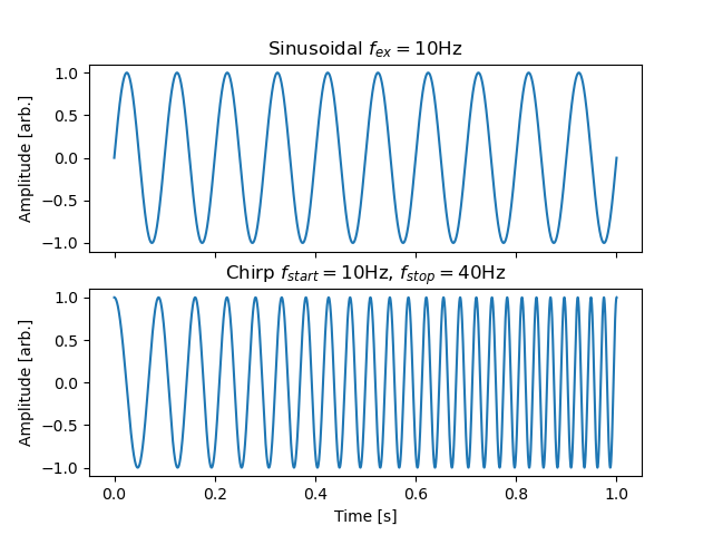
The samples can therefore be considered as a waveform sampled at the sampling frequency. To compute a sample for a sinusoidal excitation at frequency f_ex using NumPy:

samples[i] = np.sin(2*np.pi*f_ex*i/sampling_freq)

To generate the full samples array at sampling_freq sampling frequency, for n_turns turns at f_rev revolution frequency:

total_time = n_turns / f_rev
time = np.arange(0, total_time, 1/sampling_freq)
samples = np.sin(2*np.pi*f_ex*time)

To generate a chirp array at sampling_freq, between frequencies f_start and f_stop, lasting n_turns turns at f_rev revolution frequency:

chirp_time = n_turns / f_rev
time = np.arange(0, chirp_time, 1/sampling_freq)
samples = sp.signal.chirp(time, f_start, chirp_time, f_stop)

To then define an Exciter element with the custom waveform (array of samples at sampling frequency sampling freq) and normal and skew components KNL and KSL:

# Create beam element
exciter = xt.Exciter(_context = ctx,
    samples = samples,
    sampling_frequency = sampling_freq,
    duration = None,  # defaults to waveform duration
    frev = f_rev,
    start_turn = 0,  # default, seconds
    knl = KNL,
    ksl = KSL,
)

# Add it to the line for tracking as usual
line.insert_element(
    element = exciter,
    name = 'RF_KO_EXCITER',
    index = 42,
)

The optional parameter duration (seconds) may be used to repeat (or truncate) the excitation waveform. It defaults to len(samples)/sampling_freq, the duration of samples.

The element also provides the read-only parameter order, the multipole order, equal to the order of the largest non-zero multipole component knl or ksl.

Acceleration

An energy ramp with an arbitrary time dependence of the beam energy can be simulated by attaching and xtrack.EnergyProgram object to the line, as shown in the example below.

import numpy as np
from cpymad.madx import Madx
import xtrack as xt

# Import a line and build a tracker
line = xt.Line.from_json(
    '../../test_data/psb_injection/line_and_particle.json')
e_kin_start_eV = 160e6
line.particle_ref = xt.Particles(mass0=xt.PROTON_MASS_EV, q0=1.,
                                 energy0=xt.PROTON_MASS_EV + e_kin_start_eV)
line.build_tracker()

# User-defined energy ramp
t_s = np.array([0., 0.0006, 0.0008, 0.001 , 0.0012, 0.0014, 0.0016, 0.0018,
                0.002 , 0.0022, 0.0024, 0.0026, 0.0028, 0.003, 0.01])
E_kin_GeV = np.array([0.16000000,0.16000000,
    0.16000437, 0.16001673, 0.16003748, 0.16006596, 0.16010243, 0.16014637,
    0.16019791, 0.16025666, 0.16032262, 0.16039552, 0.16047524, 0.16056165,
    0.163586])

# Attach energy program to the line
line.energy_program = xt.EnergyProgram(t_s=t_s, kinetic_energy0=E_kin_GeV*1e9)

# Plot energy and revolution frequency vs time
t_plot = np.linspace(0, 10e-3, 20)
E_kin_plot = line.energy_program.get_kinetic_energy0_at_t_s(t_plot)
f_rev_plot = line.energy_program.get_frev_at_t_s(t_plot)

import matplotlib.pyplot as plt
plt.close('all')
plt.figure(1, figsize=(6.4 * 1.5, 4.8))
ax1 = plt.subplot(2,2,1)
plt.plot(t_plot * 1e3, E_kin_plot * 1e-6)
plt.ylabel(r'$E_{kin}$ [MeV]')
ax2 = plt.subplot(2,2,3, sharex=ax1)
plt.plot(t_plot * 1e3, f_rev_plot * 1e-3)
plt.ylabel(r'$f_{rev}$ [kHz]')
plt.xlabel('t [ms]')

# Setup frequency of the RF cavity  to stay on the second harmonic of the
# revolution frequency during the acceleration

t_rf = np.linspace(0, 3e-3, 100) # time samples for the frequency program
f_rev = line.energy_program.get_frev_at_t_s(t_rf)
h_rf = 2 # harmonic number
f_rf = h_rf * f_rev # frequency program

# Build a function with these samples and link it to the cavity
line.functions['fun_f_rf'] = xt.FunctionPieceWiseLinear(x=t_rf, y=f_rf)
line.element_refs['br.c02'].frequency = line.functions['fun_f_rf'](
                                                        line.vars['t_turn_s'])

# Setup voltage and lag
line.element_refs['br.c02'].voltage = 3000 # V
line.element_refs['br.c02'].lag = 0 # degrees (below transition energy)

# When setting line.vars['t_turn_s'] the reference energy and the rf frequency
# are updated automatically
line.vars['t_turn_s'] = 0
line.particle_ref.kinetic_energy0 # is 160.00000 MeV
line['br.c02'].frequency # is 1983931.935 Hz

line.vars['t_turn_s'] = 3e-3
line.particle_ref.kinetic_energy0 # is 160.56165 MeV
line['br.c02'].frequency # is 1986669.0559674294

# Back to zero for tracking!
line.vars['t_turn_s'] = 0

# Track a few particles to visualize the longitudinal phase space
p_test = line.build_particles(x_norm=0, zeta=np.linspace(0, line.get_length(), 101))

# Enable time-dependent variables (t_turn_s and all the variables that depend on
# it are automatically updated at each turn)
line.enable_time_dependent_vars = True

# Track
line.track(p_test, num_turns=9000, turn_by_turn_monitor=True, with_progress=True)
mon = line.record_last_track

# Plot
plt.subplot2grid((2,2), (0,1), rowspan=2)
plt.plot(mon.zeta[:, -2000:].T, mon.delta[:, -2000:].T, color='C0')
plt.xlabel(r'$\zeta$ [m]')
plt.ylabel('$\delta$')
plt.xlim(-40, 30)
plt.ylim(-0.0025, 0.0025)
plt.title('Last 2000 turns')
plt.subplots_adjust(left=0.08, right=0.95, wspace=0.26)
plt.show()

# Complete source: xtrack/examples/acceleration/001_energy_ramp.py

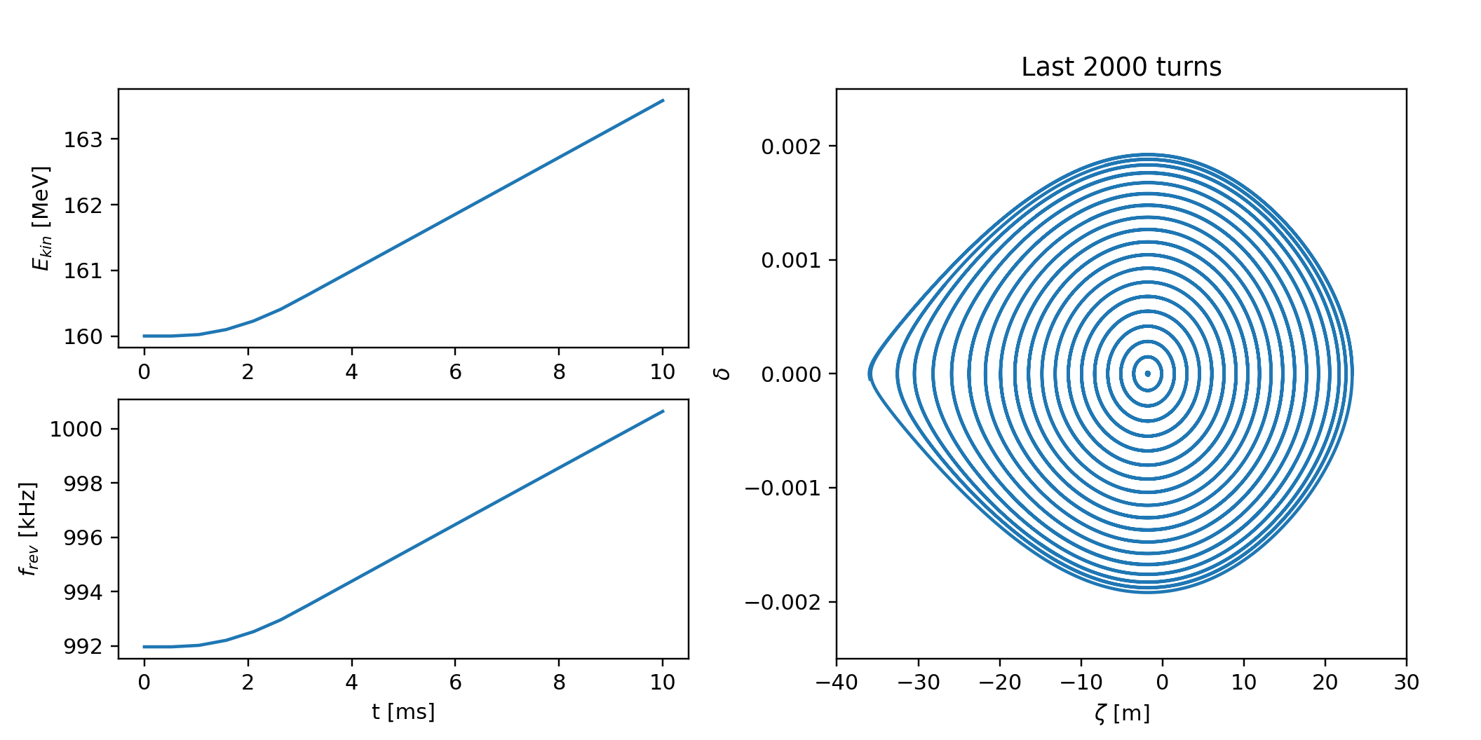
Time evolution of the beam energy and the RF frequency and particles motion in the longitudinal phase space as obtained from the example above.

Off-momentum from RF frequency change

The xtrack default RF are synchronized with the reference particle (simply because of the coordinate choice). For this reason a change of the RF frequency does not result in a change in the revolution frequency. To obtain a change in the revolution frequency (and hence in the momentum) it is necessary to introduce explicitly a time delay, using the element xtrack.ZetaShift. This is illustrated in the following example:

import numpy as np
import xtrack as xt

# Load a line and build a tracker
line = xt.Line.from_json(
    '../../test_data/hllhc15_noerrors_nobb/line_and_particle.json')
line.particle_ref = xt.Particles(mass0=xt.PROTON_MASS_EV, q0=1, energy0=7e12)
line.build_tracker()

# Frequency trim to make
df_hz = 50 # Frequency trim

# Twiss
tw0 = line.twiss()

# Compute corresponding delay to be introduced in the line:
#
# T_rev = h_rf/f_rf
# dt = h_rf/(f_rf + df_hz) - h_rf/f_rf = h_rf/f_rf (1/(1+df_hz/f_rf) - 1)
#                                       ~= h_rf/f_rf * (1 - df_hz/f_rf -1)
#                                       = -h_rf/(f_rf^2) * df_hz
#                                       = -T_rev / f_rf * df_hz
# dzeta = -beta0 * clight * dt = circumference * df_hz / f_rf

h_rf = 35640
f_rf = h_rf/tw0.T_rev0
beta0 = line.particle_ref.beta0[0]
dzeta = tw0.circumference * df_hz / f_rf

# Append delay element to the line
line.unfreeze()
line.append_element(element=xt.ZetaShift(dzeta=dzeta), name='zeta_shift')
line.build_tracker()

# Twiss
tw1 = line.twiss()

# Expected momentum from slip factor (eta = -df_rev / f_rev / delta)
f_rev = 1/tw0.T_rev0
df_rev = df_hz / h_rf
eta = tw0.slip_factor
delta_expected = -df_rev / f_rev / eta

tw1.delta[0]    # is -0.00035789
delta_expected  # is -0.00035803

# Check that particle stays off momentum in multi-turn tracking
p = tw1.particle_on_co.copy()

p_test = line.build_particles(x_norm=0,
            delta=np.linspace(delta_expected - 8e-4, delta_expected + 8e-4, 60))
# p_test = line.build_particles(x_norm=0, delta=delta_expected,
#                               zeta=np.linspace(0, 0.5, 101))

# Track
line.track(p_test, num_turns=1000, turn_by_turn_monitor=True, with_progress=True)
mon = line.record_last_track

# Plot
import matplotlib.pyplot as plt
plt.close('all')
plt.figure()
plt.plot(mon.zeta[:, :].T, mon.delta[:, :].T * 1e4, color='C0')
plt.xlabel(r'$\zeta$ [m]')
plt.ylabel('$\delta$ [$10^{-4}$]')
plt.xlim(-.8, .8)
plt.ylim(delta_expected * 1e4 - 4, delta_expected * 1e4 + 4)
plt.axhline(delta_expected * 1e4, color='r', linestyle='--',
            label='$\delta$ expected')
plt.show()

# Complete source: xtrack/examples/radial_steering/000_radial_steering.py

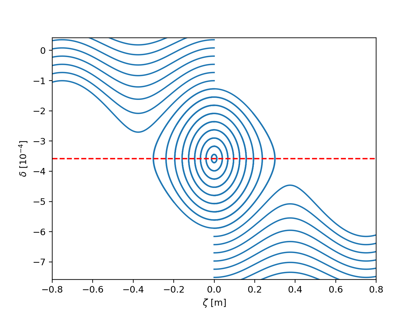
Longitudinal phase space from tracking. The backet is centered around the expected momentum.

Optimize line for multi-turn tracking speed

When the tracker is used for multi-turn tracking, the line and tracker can be optimized to increase the tracking speed. This can be done with the Line.optimize_for_tracking() method, as shown in the following example.

See also: Line.optimize_for_tracking()

import json
import time
import numpy as np

import xtrack as xt
import xpart as xp

#################################
# Load a line and build tracker #
#################################
line = xt.Line.from_json(
    '../../test_data/hllhc15_noerrors_nobb/line_w_knobs_and_particle.json')
line.particle_ref = xt.Particles(mass0=xt.PROTON_MASS_EV, p0c=7e12)
line.build_tracker()

###########################
# Generate some particles #
###########################

particles = line.build_particles(
    x_norm=np.linspace(-2, 2, 1000), y_norm=0.1, delta=3e-4,
    nemitt_x=2.5e-6, nemitt_y=2.5e-6)

p_no_optimized = particles.copy()
p_optimized = particles.copy()

##############################
# Track without optimization #
##############################

num_turns = 10
line.track(p_no_optimized, num_turns=num_turns, time=True)
t_not_optimized = line.time_last_track

####################
# Optimize tracker #
####################

line.optimize_for_tracking()

# This performs the following actions (physics model is unchanged):
# - Disables xdeps expressions
# - Removes inactive multipoles
# - Merges consecutive multipoles
# - Removes drifts with zero length
# - Merges consecutive drifts

###########################
# Track with optimization #
###########################

line.track(p_optimized, num_turns=num_turns, time=True)
t_optimized = line.time_last_track

#################
# Compare times #
#################

num_particles = len(p_no_optimized.x)
print(f'Time not optimized {t_not_optimized*1e6/num_particles/num_turns:.1f} us/part/turn')
print(f'Time optimized {t_optimized*1e6/num_particles/num_turns:.1f} us/part/turn')

###################################
# Check that result are identical #
###################################

assert np.all(p_no_optimized.state == 1)
assert np.all(p_optimized.state == 1)

assert np.allclose(p_no_optimized.x, p_optimized.x, rtol=0, atol=1e-14)
assert np.allclose(p_no_optimized.y, p_optimized.y, rtol=0, atol=1e-14)
assert np.allclose(p_no_optimized.px, p_optimized.px, rtol=0, atol=1e-14)
assert np.allclose(p_no_optimized.py, p_optimized.py, rtol=0, atol=1e-14)
assert np.allclose(p_no_optimized.zeta, p_optimized.zeta, rtol=0, atol=1e-14)
assert np.allclose(p_no_optimized.delta, p_optimized.delta, rtol=0, atol=1e-14)

# Complete source: xtrack/examples/optimized_tracker/000_optimized_tracker.py