Line
Creating a Line object
An Xsuite Line can be created by providing beam line element objects and the corresponding names, as illustrated in the following example:
import numpy as np
import xtrack as xt

# Define elements
pi = np.pi
lbend = 3
elements = {
    'mqf.1': xt.Quadrupole(length=0.3, k1=0.1),
    'd1.1':  xt.Drift(length=1),
    'mb1.1': xt.Bend(length=lbend, k0=pi / 2 / lbend, h=pi / 2 / lbend),
    'd2.1':  xt.Drift(length=1),

    'mqd.1': xt.Quadrupole(length=0.3, k1=-0.7),
    'd3.1':  xt.Drift(length=1),
    'mb2.1': xt.Bend(length=lbend, k0=pi / 2 / lbend, h=pi / 2 / lbend),
    'd4.1':  xt.Drift(length=1),

    'mqf.2': xt.Quadrupole(length=0.3, k1=0.1),
    'd1.2':  xt.Drift(length=1),
    'mb1.2': xt.Bend(length=lbend, k0=pi / 2 / lbend, h=pi / 2 / lbend),
    'd2.2':  xt.Drift(length=1),

    'mqd.2': xt.Quadrupole(length=0.3, k1=-0.7),
    'd3.2':  xt.Drift(length=1),
    'mb2.2': xt.Bend(length=lbend, k0=pi / 2 / lbend, h=pi / 2 / lbend),
    'd4.2':  xt.Drift(length=1),
}

# Build the ring
line = xt.Line(elements=elements,
               element_names=['mqf.1', 'd1.1', 'mb1.1', 'd2.1', # defines the order
                              'mqd.1', 'd3.1', 'mb2.1', 'd4.1',
                              'mqf.2', 'd1.2', 'mb1.2', 'd2.2',
                              'mqd.2', 'd3.2', 'mb2.2', 'd4.2'])
# Define reference particle
line.particle_ref = xt.Particles(p0c=1.2e9, mass0=xt.PROTON_MASS_EV)

# Complete source: xtrack/examples/toy_ring/000_toy_ring.py
Importing a line from MAD-X
An Xsuite Line object can be imported from an existing MAD-X model, through the
cpymad interface of MAD-X, using the method
xtrack.Line.from_madx_sequence(). The import of certain features of the MAD-X
model (dererred expressions, apertures, thick elements, alignment errors, field
errors, etc.) can be controlled by the user. This is illustrated in the following
example:
import numpy as np
from cpymad.madx import Madx

import xtrack as xt

import matplotlib.pyplot as plt

from cpymad.madx import Madx

mad = Madx()

# Load mad model and apply element shifts
mad.input('''
call, file = '../../test_data/psb_chicane/psb.seq';
call, file = '../../test_data/psb_chicane/psb_fb_lhc.str';

beam, particle=PROTON, pc=0.5708301551893517;
use, sequence=psb1;

select,flag=error,clear;
select,flag=error,pattern=bi1.bsw1l1.1*;
ealign, dx=-0.0057;

select,flag=error,clear;
select,flag=error,pattern=bi1.bsw1l1.2*;
select,flag=error,pattern=bi1.bsw1l1.3*;
select,flag=error,pattern=bi1.bsw1l1.4*;
ealign, dx=-0.0442;

twiss;
''')

line = xt.Line.from_madx_sequence(
    sequence=mad.sequence.psb1,
    allow_thick=True,
    enable_align_errors=True,
    deferred_expressions=True,
)
line.particle_ref = xt.Particles(mass0=xt.PROTON_MASS_EV,
                            gamma0=mad.sequence.psb1.beam.gamma)

# Complete source: xtrack/examples/psb/000a_all_xsuite_import_model.py
Define a line through a sequence
A line can also be defined through a “sequence”, providing the element s positions instead of explicit drifts, as show in the example below:
import numpy as np
from xtrack import Line, Node, Multipole

# Or from a sequence definition:
elements = {
    'quad': Multipole(length=0.3, knl=[0, +0.50]),
    'bend': Multipole(length=0.5, knl=[np.pi / 12], hxl=[np.pi / 12]),
}
sequences = {
    'arc': [Node(1.0, 'quad'), Node(4.0, 'bend', from_='quad')],
}
line = Line.from_sequence([
        Node( 0.0, 'arc'),
        Node(10.0, 'arc', name='section2'),
        Node( 3.0, Multipole(knl=[0, 0, 0.1]), from_='section2', name='sext'),
        Node( 3.0, 'quad', name='quad_5', from_='sext'),
    ], length=20,
    elements=elements, sequences=sequences,
    auto_reorder=True, copy_elements=False,
)

line.get_table().show()
# prints:
#
# name          s element_type isthick compound_name
# arc           0 Marker         False
# drift         0 Drift           True
# arcquad       1 Multipole      False
# drift1        1 Drift           True
# arcbend       5 Multipole      False
# drift2        5 Drift           True
# section2     10 Marker         False
# drift3       10 Drift           True
# section2quad 11 Multipole      False
# drift4       11 Drift           True
# sext         13 Multipole      False
# drift5       13 Drift           True
# section2bend 15 Multipole      False
# drift6       15 Drift           True
# quad_5       16 Multipole      False
# drift7       16 Drift           True
# _end_point   20                False

# Complete source: xtrack/examples/sequence/000_sequence.py
Line inspection, Line.get_table(), Line.attr[...]
The following example illustrates how to inspect the properties of a line and its elements:
import numpy as np
import xtrack as xt

pi = np.pi
lbend = 3
elements = {
    'mqf.1': xt.Quadrupole(length=0.3, k1=0.1),
    'd1.1':  xt.Drift(length=1),
    'mb1.1': xt.Bend(length=lbend, k0=pi / 2 / lbend, h=pi / 2 / lbend),
    'd2.1':  xt.Drift(length=1),

    'mqd.1': xt.Quadrupole(length=0.3, k1=-0.7),
    'd3.1':  xt.Drift(length=1),
    'mb2.1': xt.Bend(length=lbend, k0=pi / 2 / lbend, h=pi / 2 / lbend),
    'd4.1':  xt.Drift(length=1),

    'mqf.2': xt.Quadrupole(length=0.3, k1=0.1),
    'd1.2':  xt.Drift(length=1),
    'mb1.2': xt.Bend(length=lbend, k0=pi / 2 / lbend, h=pi / 2 / lbend),
    'd2.2':  xt.Drift(length=1),

    'mqd.2': xt.Quadrupole(length=0.3, k1=-0.7),
    'd3.2':  xt.Drift(length=1),
    'mb2.2': xt.Bend(length=lbend, k0=pi / 2 / lbend, h=pi / 2 / lbend),
    'd4.2':  xt.Drift(length=1),
}

# Build the ring
line = xt.Line(elements=elements, element_names=list(elements.keys()))
line.particle_ref = xt.Particles(p0c=1.2e9, mass0=xt.PROTON_MASS_EV)
line.build_tracker()

# Quick access to an element and its attributes (by name)
line['mqf.1'] # is Quadrupole(length=0.3, k1=0.1, ...)
line['mqf.1'].k1 # is 0.1
line['mqf.1'].length # is 0.3

# Quick access to an element and its attributes (by index)
line[0] # is Quadrupole(length=0.3, k1=0.1, ...)
line[0].k1 # is 0.1
line[0].length # is 0.3

# Tuple with all element names
line.element_names # is ('mqf.1', 'd1.1', 'mb1.1', 'd2.1', 'mqd.1', ...

# Tuple with all element objects
line.elements # is (Quadrupole(length=0.3, k1=0.1, ...), Drift(length=1), ...

# `line.attr[...]` can be used for efficient extraction of a given attribute for
# all elements. For example:
line.attr['length'] # is (0.3, 1, 3, 1, 0.3, 1, 3, 1, 0.3, 1, 3, 1, 0.3, 1, 3, 1)
line.attr['k1l'] # is ('0.03, 0.0, 0.0, 0.0, -0.21, 0.0, 0.0, 0.0, 0.03, ... )

# The list of all attributes can be found in
line.attr.keys() # is ('length', 'k1', 'k1l', 'k2', 'k2l', 'k3', 'k3l', 'k4', ...

# `line.get_table()`` can be used to get a table with information about the line
# elements. For example:
tab = line.get_table()

# The table can be printed
tab.show()
# prints:
#
# Table: 17 rows, 5 cols
# name          s element_type isthick compound_name
# mqf.1         0 Quadrupole      True
# d1.1        0.3 Drift           True
# mb1.1       1.3 Bend            True
# d2.1        4.3 Drift           True
# mqd.1       5.3 Quadrupole      True
# d3.1        5.6 Drift           True
# mb2.1       6.6 Bend            True
# d4.1        9.6 Drift           True
# mqf.2      10.6 Quadrupole      True
# d1.2       10.9 Drift           True
# mb1.2      11.9 Bend            True
# d2.2       14.9 Drift           True
# mqd.2      15.9 Quadrupole      True
# d3.2       16.2 Drift           True
# mb2.2      17.2 Bend            True
# d4.2       20.2 Drift           True
# _end_point 21.2                False

# Access to a single element of the table
tab['s', 'mb2.1'] # is 6.6

# Access to a single column of the table
tab['s'] # is [0.0, 0.3, 1.3, 4.3, 5.3, 5.6, 6.6, 9.6, 10.6, 10.9, 11.9, ...

# Regular expressions can be used to select elements by name
tab.rows['mb.*']
# returns:
#
# Table: 4 rows, 5 cols
# name       s element_type isthick compound_name
# mb1.1    1.3 Bend            True
# mb2.1    6.6 Bend            True
# mb1.2   11.9 Bend            True
# mb2.2   17.2 Bend            True

# Elements can be selected by type
tab.rows[tab.element_type == 'Quadrupole']
# returns:
#
# Table: 4 rows, 5 cols
# Table: 4 rows, 5 cols
# name          s element_type isthick compound_name
# mqf.1         0 Quadrupole      True
# mqd.1       5.3 Quadrupole      True
# mqf.2      10.6 Quadrupole      True
# mqd.2      15.9 Quadrupole      True

# A section of the ring can be selected using names
tab.rows['mqd.1':'mqd.2']
# returns:
#
# Table: 9 rows, 5 cols
# name          s element_type isthick compound_name
# mqd.1       5.3 Quadrupole      True
# d3.1        5.6 Drift           True
# mb2.1       6.6 Bend            True
# d4.1        9.6 Drift           True
# mqf.2      10.6 Quadrupole      True
# d1.2       10.9 Drift           True
# mb1.2      11.9 Bend            True
# d2.2       14.9 Drift           True
# mqd.2      15.9 Quadrupole      True

# A section of the ring can be selected using the s coordinate
tab.rows[3.0:7.0:'s']
# returns:
#
# Table: 4 rows, 5 cols
# name         s element_type isthick compound_name
# d2.1       4.3 Drift           True
# mqd.1      5.3 Quadrupole      True
# d3.1       5.6 Drift           True
# mb2.1      6.6 Bend            True

# A section of the ring can be selected using indexes relative one element
# (e.g. to get from three elements upstream of 'mqd.1' to two elements
# downstream of 'mb2.1')
tab.rows['mqd.1%%-3':'mb2.1%%2']
# returns:
#
# Table: 8 rows, 5 cols
# name          s element_type isthick compound_name
# d1.1        0.3 Drift           True
# mb1.1       1.3 Bend            True
# d2.1        4.3 Drift           True
# mqd.1       5.3 Quadrupole      True
# d3.1        5.6 Drift           True
# mb2.1       6.6 Bend            True
# d4.1        9.6 Drift           True
# mqf.2      10.6 Quadrupole      True

# Each of the selection methods above returns a valid table, hence selections
# can be chained. For example:
tab.rows[0:10:'s'].rows['mb.*']
# returns:
#
# Table: 2 rows, 5 cols
# name       s element_type isthick compound_name
# mb1.1    1.3 Bend            True
# mb2.1    6.6 Bend            True

# All attributes extracted by `line.attr[...]` can be included in the table
# using `attr=True`. For example, using `tab.cols[...]` to select columns, we
# we can get the focusing strength of all quadrupoles in the ring:
tab = line.get_table(attr=True)
tab.rows[tab.element_type=='Quadrupole'].cols['s length k1l']
# returns:
#
#Table: 4 rows, 4 cols
# name          s length   k1l
# mqf.1         0    0.3  0.03
# mqd.1       5.3    0.3 -0.21
# mqf.2      10.6    0.3  0.03
# mqd.2      15.9    0.3 -0.21

# Complete source: xtrack/examples/toy_ring/004_inspect.py
References and deferred expressions
Accelerators and beam lines have complex control paterns. For example, a single high-level parameter can be used to control groups of accelerator components (e.g., sets of magnets in series, groups of RF cavities, etc.) following complex dependency relations. Xsuite allows including these dependencies in the simulation model so that changes in the high-level parameters are automatically propagated down to the line elements properties. Furthermore, the dependency relations can be created, inspected and modified at run time, as illustrated in the following example:
import numpy as np
import xtrack as xt

# We build a simple ring
pi = np.pi
lbend = 3
lquad = 0.3
elements = {
    'mqf.1': xt.Quadrupole(length=lquad, k1=0.1),
    'd1.1':  xt.Drift(length=1),
    'mb1.1': xt.Bend(length=lbend, k0=pi / 2 / lbend, h=pi / 2 / lbend),
    'd2.1':  xt.Drift(length=1),

    'mqd.1': xt.Quadrupole(length=lquad, k1=-0.7),
    'd3.1':  xt.Drift(length=1),
    'mb2.1': xt.Bend(length=lbend, k0=pi / 2 / lbend, h=pi / 2 / lbend),
    'd4.1':  xt.Drift(length=1),

    'mqf.2': xt.Quadrupole(length=lquad, k1=0.1),
    'd1.2':  xt.Drift(length=1),
    'mb1.2': xt.Bend(length=lbend, k0=pi / 2 / lbend, h=pi / 2 / lbend),
    'd2.2':  xt.Drift(length=1),

    'mqd.2': xt.Quadrupole(length=lquad, k1=-0.7),
    'd3.2':  xt.Drift(length=1),
    'mb2.2': xt.Bend(length=lbend, k0=pi / 2 / lbend, h=pi / 2 / lbend),
    'd4.2':  xt.Drift(length=1),
}
line = xt.Line(elements=elements, element_names=list(elements.keys()))
line.particle_ref = xt.Particles(p0c=1.2e9, mass0=xt.PROTON_MASS_EV)

# For each quadrupole we create a variable controlling its integrated strength.
# Expressions can be associated to any beam element property, using the `element_refs`
# attribute of the line. For example:
line.vars['k1l.qf.1'] = 0
line.element_refs['mqf.1'].k1 = line.vars['k1l.qf.1'] / lquad
line.vars['k1l.qd.1'] = 0
line.element_refs['mqd.1'].k1 = line.vars['k1l.qd.1'] / lquad
line.vars['k1l.qf.2'] = 0
line.element_refs['mqf.2'].k1 = line.vars['k1l.qf.2'] / lquad
line.vars['k1l.qd.2'] = 0
line.element_refs['mqd.2'].k1 = line.vars['k1l.qd.2'] / lquad

# When a variable is changed, the corresponding element property is automatically
# updated:
line.vars['k1l.qf.1'] = 0.1
line['mqf.1'].k1 # is 0.333, i.e. 0.1 / lquad

# We can create a variable controlling the integrated strength of the two
# focusing quadrupoles
line.vars['k1lf'] = 0.1
line.vars['k1l.qf.1'] = line.vars['k1lf']
line.vars['k1l.qf.2'] = line.vars['k1lf']
# and a variable controlling the integrated strength of the two defocusing quadrupoles
line.vars['k1ld'] = -0.7
line.vars['k1l.qd.1'] = line.vars['k1ld']
line.vars['k1l.qd.2'] = line.vars['k1ld']

# Changes on the controlling variable are propagated to the two controlled ones and
# to the corresponding element properties:
line.vars['k1lf'] = 0.2
line.vars['k1l.qf.1']._get_value() # is 0.2
line.vars['k1l.qf.2']._get_value() # is 0.2
line['mqf.1'].k1 # is 0.666, i.e. 0.2 / lquad
line['mqf.2'].k1 # is 0.666, i.e. 0.2 / lquad

# The `_info()` method of a variable provides information on the existing relations
# between the variables. For example:
line.vars['k1l.qf.1']._info()
# prints:
##  vars['k1l.qf.1']._get_value()
#   vars['k1l.qf.1'] = 0.2
#
##  vars['k1l.qf.1']._expr
#   vars['k1l.qf.1'] = vars['k1lf']
#
##  vars['k1l.qf.1']._expr._get_dependencies()
#   vars['k1lf'] = 0.2
#
##  vars['k1l.qf.1']._find_dependant_targets()
#   element_refs['mqf.1'].k1

line.vars['k1lf']._info()
# prints:
##  vars['k1lf']._get_value()
#   vars['k1lf'] = 0.2
#
##  vars['k1lf']._expr is None
#
##  vars['k1lf']._find_dependant_targets()
#   vars['k1l.qf.2']
#   element_refs['mqf.2'].k1
#   vars['k1l.qf.1']
#   element_refs['mqf.1'].k1

line.element_refs['mqf.1'].k1._info()
# prints:
##  element_refs['mqf.1'].k1._get_value()
#   element_refs['mqf.1'].k1 = 0.6666666666666667
#
##  element_refs['mqf.1'].k1._expr
#   element_refs['mqf.1'].k1 = (vars['k1l.qf.1'] / 0.3)
#
##  element_refs['mqf.1'].k1._expr._get_dependencies()
#   vars['k1l.qf.1'] = 0.2
#
##  element_refs['mqf.1'].k1 does not influence any target

# Expressions can include multiple variables and mathematical operations. For example
line.vars['a'] = 3 * line.functions.sqrt(line.vars['k1lf']) + 2 * line.vars['k1ld']

# As seen above, line.vars['varname'] returns a reference object that
# can be used to build further references, or to inspect its properties.
# To get the current value of the variable, one needs to use `._get_value()`
# For quick access to the current value of a variable, one can use the `line.varval`
# attribute or its shortcut `line.vv`:
line.varval['k1lf'] # is 0.2
line.vv['k1lf']     # is 0.2
# Note an important difference when using `line.vars` or `line.varval` in building
# expressions. For example:
line.vars['a'] = 3.
line.vars['b'] = 2 * line.vars['a']
# In this case the reference to the quantity `line.vars['a']` is stored in the
# expression, and the value of `line.vars['b']` is updated when `line.vars['a']`
# changes:
line.vars['a'] = 4.
line.vv['b'] # is 8.
# On the contrary, when using `line.varval` or `line.vv` in building expressions,
# the current value of the variable is stored in the expression:
line.vv['a'] = 3.
line.vv['b'] = 2 * line.vv['a']
line.vv['b'] # is 6.
line.vv['a'] = 4.
line.vv['b'] # is still 6.

# The `line.vars.get_table()` method returns a table with the value of all the
# existing variables:
line.vars.get_table()
# returns:
#
# Table: 9 rows, 2 cols
# name     value
# t_turn_s     0
# k1l.qf.1   0.2
# k1l.qd.1  -0.7
# k1l.qf.2   0.2
# k1l.qd.2  -0.7
# k1lf       0.2
# k1ld      -0.7
# a            4
# b            6

# Regular expressions can be used to select variables. For example we can select all
# the variables containing `qf` using the following:
var_tab = line.vars.get_table()
var_tab.rows['.*qf.*']
# returns:
#
# Table: 2 rows, 2 cols
# name     value
# k1l.qf.1   0.2
# k1l.qf.2   0.2

# Complete source: xtrack/examples/toy_ring/002_expressions.py
When importing a MAD-X model, the dependency relations from MAD-X deferred expressions are automatically imported as well. The following example illustrates how to inspect the dependency relations in a line imported from MAD-X:
import xtrack as xt
import xobjects as xo

from cpymad.madx import Madx

# Load sequence in MAD-X
mad = Madx()
mad.call('../../test_data/hllhc15_noerrors_nobb/sequence.madx')
mad.use(sequence="lhcb1")

# Build Xtrack line importing MAD-X expressions
line = xt.Line.from_madx_sequence(mad.sequence['lhcb1'],
                                  deferred_expressions=True # <--
                                  )
line.particle_ref = xt.Particles(mass0=xt.PROTON_MASS_EV, q0=1,
                                 gamma0=mad.sequence.lhcb1.beam.gamma)
line.build_tracker()

# MAD-X variables can be found in `line.vars` or, equivalently, in   #
# `line.vars`. They can be used to change properties in the beamline.   #
# For example, we consider the MAD-X variable `on_x1` that controls     #
# the beam angle in the interaction point 1 (IP1). It is defined in     #
# microrad units.                                                       #

# Inspect the value of the variable
print(line.vars['on_x1']._value)
# ---> returns 1 (as defined in the import)

# Measure vertical angle at the interaction point 1 (IP1)
print(line.twiss(at_elements=['ip1'])['px'])
# ---> returns 1e-6

# Set crossing angle using the variable
line.vars['on_x1'] = 300

# Measure vertical angle at the interaction point 1 (IP1)
print(line.twiss(at_elements=['ip1'])['px'])
# ---> returns 0.00030035

# Complete source: xtrack/examples/knobs/001_lhc.py
Save and reload lines
An Xtrack Line object can be transformed into a dictionary or saved to a json file, as illustrated in the following example:
import json

import numpy as np

import xtrack as xt
import xobjects as xo

# Build a beam line
line = xt.Line(
    elements=[
        xt.Multipole(knl=np.array([1.,2.,3.])),
        xt.Drift(length=2.),
        xt.Cavity(frequency=400e9, voltage=1e6),
        xt.Multipole(knl=np.array([1.,2.,3.])),
        xt.Drift(length=2.),
    ],
    element_names=['m1', 'd1', 'c1', 'm2', 'c2']
)

# Save to json
line.to_json('line.json')

# Load from json
line_2 = xt.Line.from_json('line.json')

# Alternatively the to dict method can be used, which is more flexible for
# example to save additional information in the json file

#Save
dct = line.to_dict()
dct['my_additional_info'] = 'Important information'
with open('line.json', 'w') as fid:
    json.dump(dct, fid, cls=xo.JEncoder)

# Load
with open('line.json', 'r') as fid:
    loaded_dct = json.load(fid)
line_2 = xt.Line.from_dict(loaded_dct)
# loaded_dct['my_additional_info'] contains "Important information"

# Complete source: xtrack/examples/to_json/000_lattice_to_json.py
Element insertion
import numpy as np
import xtrack as xt

pi = np.pi
lbend = 3
elements = {
    'mqf.1': xt.Quadrupole(length=0.3, k1=0.1),
    'd1.1':  xt.Drift(length=1),
    'mb1.1': xt.Bend(length=lbend, k0=pi / 2 / lbend, h=pi / 2 / lbend),
    'd2.1':  xt.Drift(length=1),

    'mqd.1': xt.Quadrupole(length=0.3, k1=-0.7),
    'd3.1':  xt.Drift(length=1),
    'mb2.1': xt.Bend(length=lbend, k0=pi / 2 / lbend, h=pi / 2 / lbend),
    'd4.1':  xt.Drift(length=1),

    'mqf.2': xt.Quadrupole(length=0.3, k1=0.1),
    'd1.2':  xt.Drift(length=1),
    'mb1.2': xt.Bend(length=lbend, k0=pi / 2 / lbend, h=pi / 2 / lbend),
    'd2.2':  xt.Drift(length=1),

    'mqd.2': xt.Quadrupole(length=0.3, k1=-0.7),
    'd3.2':  xt.Drift(length=1),
    'mb2.2': xt.Bend(length=lbend, k0=pi / 2 / lbend, h=pi / 2 / lbend),
    'd4.2':  xt.Drift(length=1),
}

# Build the ring
line = xt.Line(elements=elements, element_names=list(elements.keys()))
line.particle_ref = xt.Particles(p0c=1.2e9, mass0=xt.PROTON_MASS_EV)
line.build_tracker()

# Inspect the line
tab = line.get_table()
tab.show()
# prints:
#
# Table: 17 rows, 5 cols
# name          s element_type isthick compound_name
# mqf.1         0 Quadrupole      True
# d1.1        0.3 Drift           True
# mb1.1       1.3 Bend            True
# d2.1        4.3 Drift           True
# mqd.1       5.3 Quadrupole      True
# d3.1        5.6 Drift           True
# mb2.1       6.6 Bend            True
# d4.1        9.6 Drift           True
# mqf.2      10.6 Quadrupole      True
# d1.2       10.9 Drift           True
# mb1.2      11.9 Bend            True
# d2.2       14.9 Drift           True
# mqd.2      15.9 Quadrupole      True
# d3.2       16.2 Drift           True
# mb2.2      17.2 Bend            True
# d4.2       20.2 Drift           True
# _end_point 21.2                False

# Define a sextupole
my_sext = xt.Sextupole(length=0.1, k2=0.1)
# Insert copies of the defined sextupole downstream of the quadrupoles
line.discard_tracker() # needed to modify the line structure
line.insert_element('msf.1', my_sext.copy(), at_s=tab['s', 'mqf.1'] + 0.4)
line.insert_element('msd.1', my_sext.copy(), at_s=tab['s', 'mqd.1'] + 0.4)
line.insert_element('msf.2', my_sext.copy(), at_s=tab['s', 'mqf.2'] + 0.4)
line.insert_element('msd.2', my_sext.copy(), at_s=tab['s', 'mqd.2'] + 0.4)

# Define a rectangular aperture
my_aper = xt.LimitRect(min_x=-0.02, max_x=0.02, min_y=-0.01, max_y=0.01)
# Insert the aperture upstream of the first bending magnet
line.insert_element('aper', my_aper, index='mb1.1')

line.get_table().show()
# prints:
#
# name          s element_type isthick compound_name
# mqf.1         0 Quadrupole      True
# d1.1_u      0.3 Drift           True
# msf.1       0.4 Sextupole       True
# d1.1_d      0.5 Drift           True
# aper        1.3 LimitRect      False
# mb1.1       1.3 Bend            True
# d2.1        4.3 Drift           True
# mqd.1       5.3 Quadrupole      True
# d3.1_u      5.6 Drift           True
# msd.1       5.7 Sextupole       True
# d3.1_d      5.8 Drift           True
# mb2.1       6.6 Bend            True
# d4.1        9.6 Drift           True
# mqf.2      10.6 Quadrupole      True
# d1.2_u     10.9 Drift           True
# msf.2        11 Sextupole       True
# d1.2_d     11.1 Drift           True
# mb1.2      11.9 Bend            True
# d2.2       14.9 Drift           True
# mqd.2      15.9 Quadrupole      True
# d3.2_u     16.2 Drift           True
# msd.2      16.3 Sextupole       True
# d3.2_d     16.4 Drift           True
# mb2.2      17.2 Bend            True
# d4.2       20.2 Drift           True
# _end_point 21.2                False

# Complete source: xtrack/examples/toy_ring/005_insert_element.py
Element slicing
It is possible to slice thick element with thin or thick slices, using the Uniform or the Teapot scheme. This is illustrated in the following example:
import numpy as np
import xtrack as xt

# We build a simple ring
pi = np.pi
lbend = 3
lquad = 0.3
elements = {
    'mqf.1': xt.Quadrupole(length=lquad, k1=0.1),
    'msf.1': xt.Sextupole(length=0.1, k2=0.),
    'd1.1':  xt.Drift(length=0.9),
    'mb1.1': xt.Bend(length=lbend, k0=pi / 2 / lbend, h=pi / 2 / lbend),
    'd2.1':  xt.Drift(length=1),

    'mqd.1': xt.Quadrupole(length=lquad, k1=-0.7),
    'd3.1':  xt.Drift(length=1),
    'mb2.1': xt.Bend(length=lbend, k0=pi / 2 / lbend, h=pi / 2 / lbend),
    'd4.1':  xt.Drift(length=1),

    'mqf.2': xt.Quadrupole(length=lquad, k1=0.1),
    'd1.2':  xt.Drift(length=1),
    'mb1.2': xt.Bend(length=lbend, k0=pi / 2 / lbend, h=pi / 2 / lbend),
    'd2.2':  xt.Drift(length=1),

    'mqd.2': xt.Quadrupole(length=lquad, k1=-0.7),
    'd3.2':  xt.Drift(length=1),
    'mb2.2': xt.Bend(length=lbend, k0=pi / 2 / lbend, h=pi / 2 / lbend),
    'd4.2':  xt.Drift(length=1),
}
line = xt.Line(elements=elements, element_names=list(elements.keys()))
line.particle_ref = xt.Particles(p0c=1.2e9, mass0=xt.PROTON_MASS_EV)

line_before_slicing = line.copy() # Keep for comparison

# Slice different elements with different strategies (in case multiple strategies
# apply to the same element, the last one takes precedence)
line.slice_thick_elements(
    slicing_strategies=[
        # Slicing with thin elements
        xt.Strategy(slicing=xt.Teapot(1)), # (1) Default applied to all elements
        xt.Strategy(slicing=xt.Uniform(2), element_type=xt.Bend), # (2) Selection by element type
        xt.Strategy(slicing=xt.Teapot(3), element_type=xt.Quadrupole),  # (4) Selection by element type
        xt.Strategy(slicing=xt.Teapot(4), name='mb1.*'), # (5) Selection by name pattern
        # Slicing with thick elements
        xt.Strategy(slicing=xt.Uniform(2, mode='thick'), name='mqf.*'), # (6) Selection by name pattern
        # Do not slice (leave untouched)
        xt.Strategy(slicing=None, name='mqd.1') # (7) Selection by name
    ])
line.build_tracker()
line_before_slicing.build_tracker()

# Ispect the result:

ltable = line.get_table(attr=True).cols['s', 'isthick', 'element_type']

# The sextupole msf.1 has one thin slice, as default strategy (1) is applied.
ltable.rows['msf.1_entry':'msf.1_exit']
# returns:
#
# Table: 5 rows, 4 cols
# name              s isthick element_type
# msf.1_entry     0.3   False Marker
# drift_msf.1..0  0.3    True Drift
# msf.1..0       0.35   False Multipole
# drift_msf.1..1 0.35    True Drift
# msf.1_exit      0.4   False Marker

# The bend mb2.1 has three thin slices, as strategy (2) is applied.
ltable.rows['mb2.1_entry':'mb2.1_exit']
# returns:
#
# Table: 7 rows, 4 cols
# name             s isthick element_type
# mb2.1_entry    6.6   False Marker
# drift_mb2.1..0 6.6    True Drift
# mb2.1..0       7.6   False Multipole
# drift_mb2.1..1 7.6    True Drift
# mb2.1..1       8.6   False Multipole
# drift_mb2.1..2 8.6    True Drift
# mb2.1_exit     9.6   False Marker

# The quadrupole mqd.2 has four thin slices, as strategy (3) is applied.
ltable.rows['mqd.2_entry':'mqd.2_exit']
# returns:
#
# Table: 7 rows, 4 cols
# name             s isthick element_type
# mb2.1_entry    6.6   False Marker
# drift_mb2.1..0 6.6    True Drift
# mb2.1..0       7.6   False Multipole
# drift_mb2.1..1 7.6    True Drift
# mb2.1..1       8.6   False Multipole
# drift_mb2.1..2 8.6    True Drift
# mb2.1_exit     9.6   False Marker

# The quadrupole mqf.1 has two thick slices, as strategy (6) is applied.
ltable.rows['mqf.1_entry':'mqf.1_exit']
# returns:
#
# Table: 4 rows, 4 cols
# name              s isthick element_type
# mqf.1_entry       0   False Marker
# mqf.1..0          0    True Quadrupole
# mqf.1..1       0.15    True Quadrupole
# mqf.1_exit      0.3   False Marker

# The quadrupole mqd.1 is left untouched, as strategy (7) is applied.
ltable.rows['mqd.1']
# returns:
#
# Table: 1 row, 4 cols
# name             s isthick element_type
# mqd.1          5.3    True Quadrupole

# Complete source: xtrack/examples/toy_ring/003_slicing.py
Simulation of small rings: drifts, bends, fringe fields
By default, Xsuite uses and expanded Hamiltonian formalism for the bend and the drift and well as linearized maps for the dipole edges. For small rings featuring large bending angles it is advisable to switch to the full model for the bends, the fringe fields and the drifts (note, instead, that for large rings the expanded Hamiltonian formalism is more efficient and accurate).
The following example illustrates how to switch to the full model for the bends, the fringe fields and the drifts and compares the effect of the two models on the optics functions and the chromatic properties of the CERN ELENA ring:
import numpy as np
from cpymad.madx import Madx
import xtrack as xt

# We get the model from MAD-X
mad = Madx()
folder = ('../../test_data/elena')
mad.call(folder + '/elena.seq')
mad.call(folder + '/highenergy.str')
mad.call(folder + '/highenergy.beam')
mad.use('elena')

# Build xsuite line
seq = mad.sequence.elena
line = xt.Line.from_madx_sequence(seq)
line.particle_ref = xt.Particles(gamma0=seq.beam.gamma,
                                    mass0=seq.beam.mass * 1e9,
                                    q0=seq.beam.charge)

# Inspect one bend (the bend is a compound element made by a core and two edge elements)
tt = line.get_table()
tt.rows['lnr.mbhek.0135_entry':'lnr.mbhek.0135_exit'].show()
# name                          s element_type isthick ...
# lnr.mbhek.0135_entry     4.4992 Marker         False
# lnr.mbhek.0135_den       4.4992 DipoleEdge     False
# lnr.mbhek.0135           4.4992 Bend            True
# lnr.mbhek.0135_dex      5.46995 DipoleEdge     False
# lnr.mbhek.0135_exit     5.46995 Marker         False

# By default the expanded model is used for the core and the linearized model for the edge
line['lnr.mbhek.0135'].model # is 'expanded'
line['lnr.mbhek.0135_den'].model # is 'linear'

# For small machines (bends with large bending angles) it is more appropriate to
# switch to the `full` model for the core and the edge
line.configure_bend_model(core='full', edge='full')

# It is also possible to switch from the expanded drift to the exact one
line.config.XTRACK_USE_EXACT_DRIFTS = True

line['lnr.mbhek.0135'].model # is 'full'
line['lnr.mbhek.0135_den'].model # is 'full'

# Slice the bends to see the behavior of the optics functions within them
line.slice_thick_elements(
    slicing_strategies=[
        xt.Strategy(slicing=None), # don't touch other elements
        xt.Strategy(slicing=xt.Uniform(10, mode='thick'), element_type=xt.Bend)
    ])

# Twiss
tw = line.twiss(method='4d')

# Switch back to the default model
line.configure_bend_model(core='expanded', edge='linear')
line.config.XTRACK_USE_EXACT_DRIFTS = False

# Twiss with the default model
tw_simpl = line.twiss(method='4d')

# Compare beta functions and chromatic properties

import matplotlib.pyplot as plt
plt.close('all')
plt.figure(1, figsize=(6.4, 4.8 * 1.5))
ax1 = plt.subplot(4,1,1)
plt.plot(tw.s, tw.betx, label='full')
plt.plot(tw_simpl.s, tw_simpl.betx, '--', label='simplified')
plt.ylabel(r'$\beta_x$')
plt.legend(loc='best')

ax2 = plt.subplot(4,1,2, sharex=ax1)
plt.plot(tw.s, tw.bety)
plt.plot(tw_simpl.s, tw_simpl.bety, '--')
plt.ylabel(r'$\beta_y$')

ax3 = plt.subplot(4,1,3, sharex=ax1)
plt.plot(tw.s, tw.wx_chrom)
plt.plot(tw_simpl.s, tw_simpl.wx_chrom, '--')
plt.ylabel(r'$W_x$')

ax4 = plt.subplot(4,1,4, sharex=ax1)
plt.plot(tw.s, tw.wy_chrom)
plt.plot(tw_simpl.s, tw_simpl.wy_chrom, '--')
plt.ylabel(r'$W_y$')
plt.xlabel('s [m]')

# Highlight the bends
tt_sliced = line.get_table()
tbends = tt_sliced.rows[tt_sliced.element_type == 'Bend']
for ax in [ax1, ax2, ax3, ax4]:
    for nn in tbends.name:
        ax.axvspan(tbends['s', nn], tbends['s', nn] + line[nn].length,
                   color='b', alpha=0.2, linewidth=0)

plt.show()

# Complete source: xtrack/examples/small_rings/000_elena_chromatic_functions.py
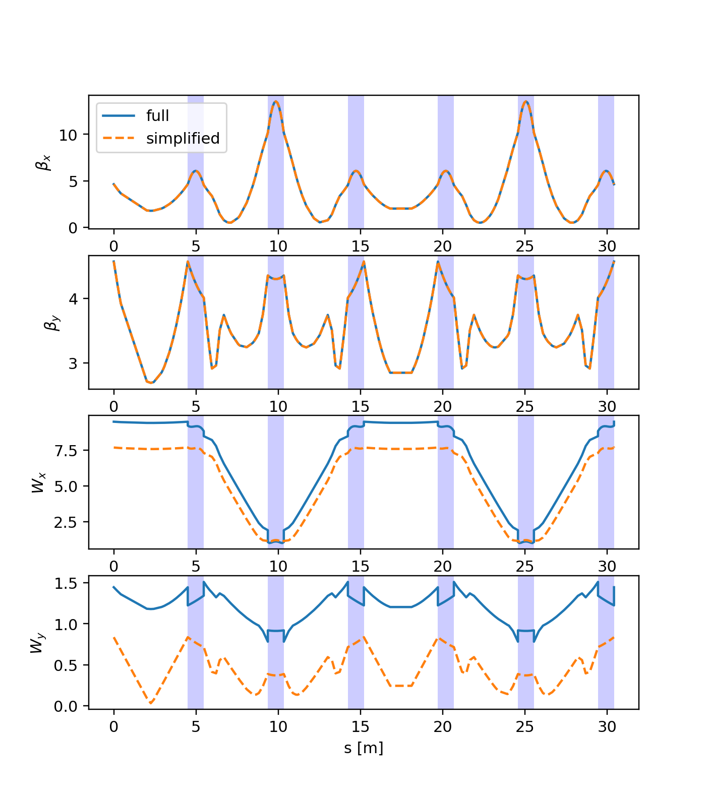
Comparison of the simplified and full model for the CERN ELENA ring (the six bends of the ring are highlighted in blue). While the linear optics is well reproduced by the simplified model, the chromatic properties differ significantly (in particular, note the effect of the dipole edges).
Extraction of second order transfer maps
The method xtrack.Line.get_line_with_second_order_maps() allows modeling portions
of a beam line with second order transfer maps. This is illustrated in the
following example.
See also xtrack.SecondOrderTaylorMap.from_line().
import numpy as np
import xtrack as xt

# Get a line and build a tracker
line = xt.Line.from_json('../../test_data/hllhc15_thick/lhc_thick_with_knobs.json')
line.build_tracker()

# Switch RF on
line.vars['vrf400'] = 16
line.vars['lagrf400.b1'] = 0.5

# Enable crossing angle orbit bumps
line.vars['on_x1'] = 10
line.vars['on_x2'] = 20
line.vars['on_x5'] = 10
line.vars['on_x8'] = 30

# Generate line made on maps (splitting at defined markers)
ele_cut = ['ip1', 'ip2', 'ip5', 'ip8'] # markers where to split the line
line_maps = line.get_line_with_second_order_maps(split_at=ele_cut)
line_maps.build_tracker()

line_maps.get_table().show()
# prints:
#
# name              s element_type         isthick compound_name
# ip7               0 Marker                 False
# map_0             0 SecondOrderTaylorMap    True
# ip8         3321.22 Marker                 False
# map_1       3321.22 SecondOrderTaylorMap    True
# ip1         6664.72 Marker                 False
# map_2       6664.72 SecondOrderTaylorMap    True
# ip2         9997.16 Marker                 False
# map_3       9997.16 SecondOrderTaylorMap    True
# ip5           19994 Marker                 False
# map_4         19994 SecondOrderTaylorMap    True
# lhcb1ip7_p_ 26658.9 Marker                 False
# _end_point  26658.9                        False

# Compare twiss of the two lines
tw = line.twiss()
tw_map = line_maps.twiss()

tw.qx       # is 62.3099999
tw_map.qx   # is  0.3099999

tw.dqx      # is 1.9135
tw_map.dqx  # is 1.9137

tw.rows[['ip1', 'ip2', 'ip5', 'ip8']].cols['x px y py betx bety'].show()
# prints
#
# name           x          px           y          py    betx    bety
# ip8  9.78388e-09 3.00018e-05 6.25324e-09 5.47624e-09 1.50001 1.49999
# ip1  1.92278e-10 1.00117e-05 2.64869e-09  1.2723e-08    0.15    0.15
# ip2  1.47983e-08 2.11146e-09 -2.1955e-08 2.00015e-05      10 9.99997
# ip5 -3.03593e-09 5.75413e-09 5.13184e-10  1.0012e-05    0.15    0.15

tw_map.rows[['ip1', 'ip2', 'ip5', 'ip8']].cols['x px y py betx bety']
# prints
#
# name             x          px           y          py    betx    bety
# ip8    9.78388e-09 3.00018e-05 6.25324e-09 5.47624e-09 1.50001 1.49999
# ip1    1.92278e-10 1.00117e-05 2.64869e-09  1.2723e-08    0.15    0.15
# ip2    1.47983e-08 2.11146e-09 -2.1955e-08 2.00015e-05      10 9.99997
# ip5   -3.03593e-09 5.75413e-09 5.13184e-10  1.0012e-05    0.15    0.15

# Complete source: xtrack/examples/taylor_map/000_line_with_maps.py