Reference guide
Beam elements (xtrack)
Marker
- class xtrack.Marker(*args, **kwargs)
A marker beam element with no effect on the particles.
Drift
- class xtrack.Drift(length=None, model=None, **kwargs)
Beam element modeling a drift section.
- Parameters:
length (float) – Length of the drift section in meters. Default is
0.model (str) – Model used for the drift element. Available models are: “adaptive”, “expanded”, “exact”. Default is “adaptive”.
Notes
Additional information on the definition of element properties and the implemented physics and models can be found in the Xsuite physics guide (https://xsuite.readthedocs.io/en/latest/physicsguide.html).
- static get_available_models()
Get list of available models for this element.
- Returns:
List of available models.
- Return type:
List[str]
Bend
- class xtrack.Bend(**kwargs)
Bending magnet element, sector-bend type.
- Parameters:
length (float) – Length of the element in meters along the reference trajectory.
angle (float) – Angle of the bend in radians. This is the angle by which the reference trajectory is bent in the horizontal plane.
k0 (float, optional) – Strength of the horizontal dipolar component in units of m^-1. It can be set to the string value ‘from_h’, in which case k0 is computed from the curvature defined by angle and length (i.e. k0 = h = angle/length) and k0_from_h is set to True.
k1 (float, optional) – Strength of the quadrupolar component in units of m^-2.
k2 (float, optional) – Strength of the sextupolar component in units of m^-3.
k0_from_h (bool, optional) – If True, k0 is computed from the curvature defined by angle and length (i.e. k0 = h = angle/length). Default is True. The flag becomes false when k0 is set directly to a numeric value.
knl (array-like) – Integrated strengths of additional normal multipole components in m^(-order).
ksl (array-like) – Integrated strengths of additional skew multipole components in m^(-order).
order (int) – Maximum order of additional multipole components. Default is
5.knl_rel (array, optional) – Relative integrated strength of the normal components with respect to the main component k0. The effect of knl_rel is added to the one of knl.
ksl_rel (array, optional) – Relative integrated strength of the skew components with respect to the main component k0. The effect of ksl_rel is added to the one of ksl.
model (str) – Model used for the element. Available models are: “adaptive”, “bend-kick-bend”, “rot-kick-rot”, “mat-kick-mat”, “drift-kick-drift-exact”, “drift-kick-drift-expanded”. Default is “adaptive”.
integrator (str) – Integrator used for the element. Available integrators are: “adaptive”, “teapot”, “yoshida4”, “uniform”. Default is “adaptive”.
num_multipole_kicks (int) – Number of multipole kicks to be used. For the yoshida integrator, this is rounded up to the nearest number compatible with the integrator scheme. Default is
0, for which the number of kicks is chosen automatically based on the element length and strength.edge_entry_active (bool) – Edge effects at the entrance edge are active if True. Default is True.
edge_exit_active (bool) – Edge effects at the exit edge are active if True. Default is True.
edge_entry_model (str) – Model used for the entrance edge. Available models are: “suppressed”, “linear”, “full”, “dipole-only”. Default is “linear”.
edge_exit_model (str) – Model used for the exit edge. Available models are: “suppressed”, “linear”, “full”, “dipole-only”. Default is “linear”.
edge_entry_angle (float) – Entrance edge angle in radians. Default is
0.edge_exit_angle (float) – Exit edge angle in radians. Default is
0.edge_entry_angle_fdown (float) – Angle of the reference trajectory at the entrance edge. Used only when edge_entry_model is “linear”. Default is
0.edge_exit_angle_fdown (float) – Angle of the reference trajectory at the exit edge. Used only when edge_exit_model is “linear”. Default is
0.edge_entry_fint (float) – Fringe field integral at the entrance edge. Used only when edge_entry_model is “full”. Default is
0.edge_exit_fint (float) – Fringe field integral at the exit edge. Used only when edge_exit_model is “full”. Default is
0.shift_x (float) – Horizontal shift of the element in meters. Default is
0.shift_y (float) – Vertical shift of the element in meters. Default is
0.shift_s (float) – Longitudinal shift of the element in meters. Default is
0.rot_s_rad (float) – Rotation around the longitudinal axis in radians. Default is
0.rot_x_rad (float) – Rotation around the horizontal axis in radians. Default is
0.rot_y_rad (float) – Rotation around the vertical axis in radians. Default is
0.rot_s_rad_no_frame (float) – Additional rotation around the longitudinal axis in radians. In this case the element field is rotated, but the reference frame at the interfaces is not changed. Default is
0.rot_shift_anchor (float) – Position along the element length where the rotations and shifts are applied. Given in meters from the element entrance. Default is
0.
Notes
Additional information on the definition of element properties and the implemented physics and models can be found in the Xsuite physics guide (https://xsuite.readthedocs.io/en/latest/physicsguide.html).
- property main_strength
Integrated strength of the main dipole component k0*length.
The definition of the misalignment parameters (rot_s_rad,
rot_s_rad_no_frame, rot_x_rad, rot_y_rad, shift_x, shift_y, shift_s)
can be found in the element misalignment section.
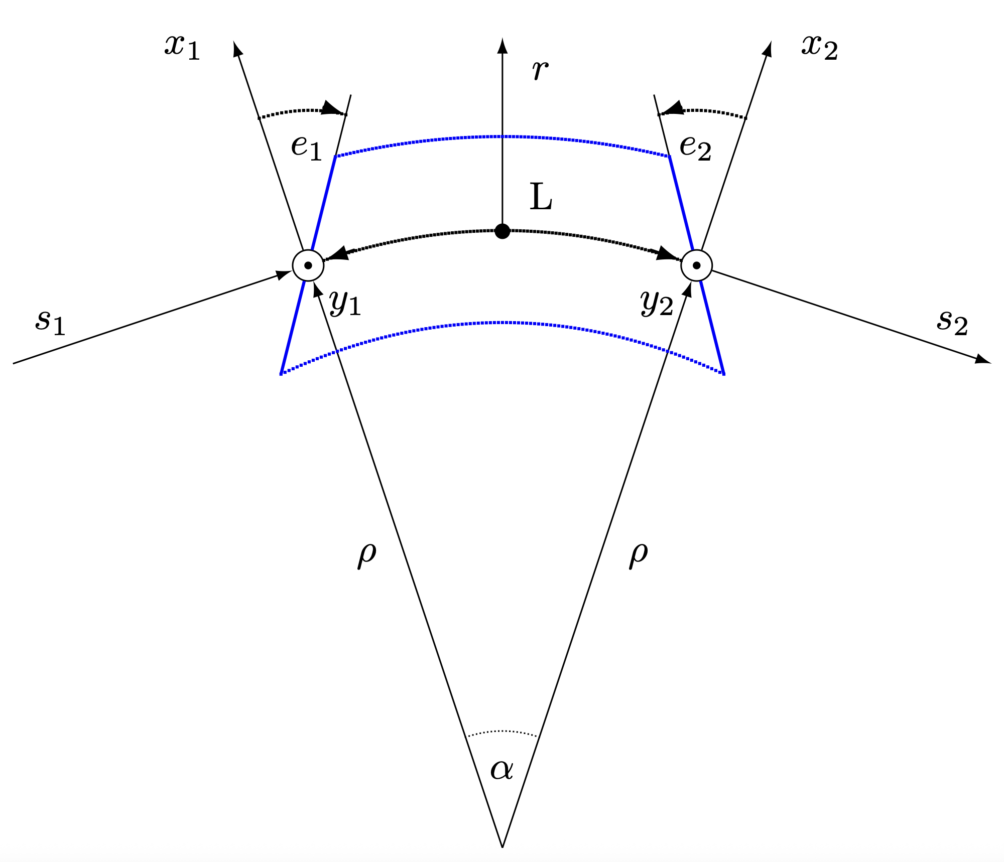
Sector bend (figure from MAD-X manual).
Symbol |
Xsuite attribute name |
|---|---|
\(L\) |
|
\(\alpha\) |
|
\(h = 1/\rho\) |
|
\(e_1\) |
|
\(e_2\) |
|
RBend
- class xtrack.RBend(**kwargs)
Rectangular bending magnet element.
- Parameters:
length_strait (float) – Length of the element in meters along the axis of the magnet (straight line between entry and exit points). This is different from the length of the reference trajectory, i.e. the increase of the s coordinate through the element, which is computed internally and can be inspected via the length property.
angle (float) – Angle of the bend in radians. This is the angle by which the reference trajectory is bent in the horizontal plane.
k0 (float) – Strength of the horizontal dipolar component in units of m^-1. It can be set to the string value ‘from_h’, in which case k0 is computed from the curvature defined by angle and length (i.e. k0 = h = angle/length) and k0_from_h is set to True.
k1 (float) – Strength of the quadrupolar component in units of m^-2.
k2 (float) – Strength of the sextupolar component in units of m^-3.
k0_from_h (bool) – If True, k0 is computed from the curvature defined by angle and length (i.e. k0 = h = angle/length). Default is True. The flag becomes false when k0 is set directly to a numeric value.
rbend_model (str) – Model used for the rectangular bend. Possible values are: “adaptive’, “curved-body”, “straight-body”. Default is “adaptive’, which falls back to “curved-body”.
rbend_angle_diff (float) – Difference in radians between the angle of the reference trajectory with respect to the magnet axis at the entrance and exit of the magnet. See drawing on Xsuite Physics Guide. Default is 0.0.
rbend_shift (float) – Shift of the magnet body, in meters, defined as the displacement of the reference trajectory with respect to the magnet axis at the center of the magnet. This parameter has effect only when rbend_model is “straight-body”. Default is 0.0.
rbend_compensate_sagitta (bool) – If True, the magnet body is shifted by half of the trajectory sagitta, defined as (1 / h) * (1 - cos(angle / 2)). The shift is added to rbend_shift. This parameter has effect only when rbend_model is “straight-body”. Default is True.
knl (array-like) – Integrated strengths of additional normal multipole components in m^(-order).
ksl (array-like) – Integrated strengths of additional skew multipole components in m^(-order).
order (int) – Maximum order of additional multipole components. Default is
5.knl_rel (array) – Relative integrated strength of the normal components with respect to the main component k0. The effect of knl_rel is added to the one of knl.
ksl_rel (array) – Relative integrated strength of the skew components with respect to the main component k0. The effect of ksl_rel is added to the one of ksl.
model (str) – Model used for the element. Available models are: “adaptive”, “bend-kick-bend”, “rot-kick-rot”, “mat-kick-mat”, “drift-kick-drift-exact”, “drift-kick-drift-expanded”. Default is “adaptive”.
integrator (str) – Integrator used for the element. Available integrators are: “adaptive”, “teapot”, “yoshida4”, “uniform”. Default is “adaptive”.
num_multipole_kicks (int) – Number of multipole kicks to be used. For the yoshida integrator, this is rounded up to the nearest number compatible with the integrator scheme. Default is
0, for which the number of kicks is chosen automatically based on the element length and strength.edge_entry_active (bool) – Edge effects at the entrance edge are active if True. Default is True.
edge_exit_active (bool) – Edge effects at the exit edge are active if True. Default is True.
edge_entry_model (str) – Model used for the entrance edge. Available models are: “suppressed”, “linear”, “full”, “dipole-only”. Default is “linear”.
edge_exit_model (str) – Model used for the exit edge. Available models are: “suppressed”, “linear”, “full”, “dipole-only”. Default is “linear”.
edge_entry_angle (float) – Entrance edge angle in radians. Default is
0.edge_exit_angle (float) – Exit edge angle in radians. Default is
0.edge_entry_angle_fdown (float) – Angle of the reference trajectory at the entrance edge. Used only when edge_entry_model is “linear”. Default is
0.edge_exit_angle_fdown (float) – Angle of the reference trajectory at the exit edge. Used only when edge_exit_model is “linear”. Default is
0.edge_entry_fint (float) – Fringe field integral at the entrance edge. Used only when edge_entry_model is “full”. Default is
0.edge_exit_fint (float) – Fringe field integral at the exit edge. Used only when edge_exit_model is “full”. Default is
0.shift_x (float) – Horizontal shift of the element in meters. Default is
0.shift_y (float) – Vertical shift of the element in meters. Default is
0.shift_s (float) – Longitudinal shift of the element in meters. Default is
0.rot_s_rad (float) – Rotation around the longitudinal axis in radians. Default is
0.rot_x_rad (float) – Rotation around the horizontal axis in radians. Default is
0.rot_y_rad (float) – Rotation around the vertical axis in radians. Default is
0.rot_s_rad_no_frame (float) – Additional rotation around the longitudinal axis in radians. In this case the element field is rotated, but the reference frame at the interfaces is not changed. Default is
0.rot_shift_anchor (float) – Position along the element length where the rotations and shifts are applied. Given in meters from the element entrance. Default is
0.
Notes
Additional information on the definition of element properties and the implemented physics and models can be found in the Xsuite physics guide (https://xsuite.readthedocs.io/en/latest/physicsguide.html).
- property main_strength
Integrated strength of the main dipole component k0*length.
The definition of the misalignment parameters (rot_s_rad,
rot_s_rad_no_frame, rot_x_rad, rot_y_rad, shift_x, shift_y, shift_s)
can be found in the element misalignment section.
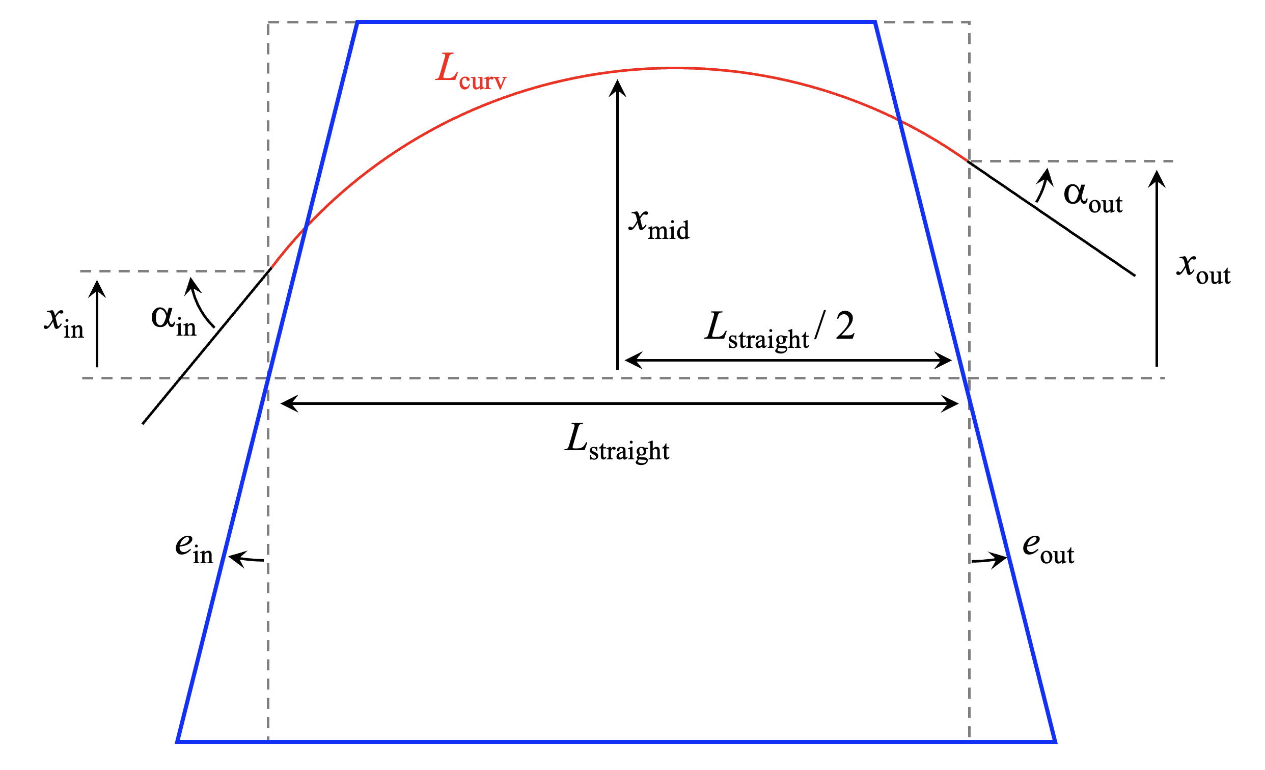
Rectangular with arbitrary face angles and arbitrary placement with respect to the reference trajectory.
Symbol |
Xsuite attribute name |
|---|---|
\(L_\text{straight}\) |
|
\(L_\text{curv}\) |
|
\(\alpha = \alpha_\text{in} + \alpha_\text{out}\) |
|
\(\alpha_\text{diff} = \alpha_\text{out} - \alpha_\text{in}\) |
|
\(x_\text{mid}\) |
|
\(e_1\) |
|
\(e_2\) |
|
Quadrupole
- class xtrack.Quadrupole(**kwargs)
Quadrupole element.
- Parameters:
k1 (float) – Strength of the quadrupole component in m^-2.
k1s (float) – Strength of the skew quadrupole component in m^-2.
length (float) – Length of the element in meters.
knl (array-like) – Integrated strengths of additional normal multipole components in m^(-order).
ksl (array-like) – Integrated strengths of additional skew multipole components in m^(-order).
order (int) – Maximum order of additional multipole components. Default is
5.knl_rel (array, optional) – Relative integrated strength of the normal components with respect to the main component k1 or k1s, depending whether main_is_skew is False or True, respectively. The effect of knl_rel is added to the one of knl.
ksl_rel (array, optional) – Relative integrated strength of the skew components with respect to the main component k1 or k1s, depending whether main_is_skew is False or True, respectively. The effect of ksl_rel is added to the one of ksl.
main_is_skew (bool, optional) – If True, the main component is the skew one (k1s), otherwise it is the normal one (k1). Default is False.
model (str) – Model used for the element. Available models are: “adaptive”, “mat-kick-mat”, “drift-kick-drift-exact”, “drift-kick-drift-expanded”. Default is “adaptive”.
integrator (str) – Integrator used for the element. Available integrators are: “adaptive”, “teapot”, “yoshida4”, “uniform”. Default is “adaptive”.
num_multipole_kicks (int) – Number of multipole kicks to be used. For the yoshida integrator, this is rounded up to the nearest number compatible with the integrator scheme. Default is
0, for which the number of kicks is chosen automatically based on the element length and strength.edge_entry_active (bool) – Fringe field at the entrance edge is active if True. Default is False.
edge_exit_active (bool) – Fringe field at the exit edge is active if True. Default is False.
shift_x (float) – Horizontal shift of the element in meters. Default is
0.shift_y (float) – Vertical shift of the element in meters. Default is
0.shift_s (float) – Longitudinal shift of the element in meters. Default is
0.rot_s_rad (float) – Rotation around the longitudinal axis in radians. Default is
0.rot_x_rad (float) – Rotation around the horizontal axis in radians. Default is
0.rot_y_rad (float) – Rotation around the vertical axis in radians. Default is
0.rot_s_rad_no_frame (float) – Additional rotation around the longitudinal axis in radians. In this case the element field is rotated, but the reference frame at the interfaces is not changed. Default is
0.rot_shift_anchor (float) – Position along the element length where the rotations and shifts are applied. Given in meters from the element entrance. Default is
0.
Notes
Additional information on the definition of element properties and the implemented physics and models can be found in the Xsuite physics guide (https://xsuite.readthedocs.io/en/latest/physicsguide.html).
- property main_strength
Returns the integrated strength of the main component, i.e. k1*length if the main component is the normal one, or k1s*length if the main component is the skew one.
- property main_is_skew
It is True if the main component is the skew one, i.e. k1s, or False if the main component is the normal one, i.e. k1.
- static get_available_integrators()
Get list of available integrators for this element.
- Returns:
List of available integrators.
- Return type:
List[str]
- static get_available_models()
Get list of available models for this element.
- Returns:
List of available models.
- Return type:
List[str]
The definition of the misalignment parameters (rot_s_rad,
rot_s_rad_no_frame, rot_x_rad, rot_y_rad, shift_x, shift_y, shift_s)
can be found in the element misalignment section.
Sextupole
- class xtrack.Sextupole(**kwargs)
Sextupole element.
- Parameters:
k2 (float) – Strength of the sextupole component in m^-3.
k2s (float) – Strength of the skew sextupole component in m^-3.
length (float) – Length of the element in meters.
knl (array-like) – Integrated strengths of additional normal multipole components in m^(-order).
ksl (array-like) – Integrated strengths of additional skew multipole components in m^(-order).
order (int) – Maximum order of additional multipole components. Default is
5.knl_rel (array, optional) – Relative integrated strength of the normal components with respect to the main component k2 or k2s, depending on whether main_is_skew is False or True, respectively. The effect of knl_rel is added to the one of knl.
ksl_rel (array, optional) – Relative integrated strength of the skew components with respect to the main component k2 or k2s, depending on whether main_is_skew is False or True, respectively. The effect of ksl_rel is added to the one of ksl.
main_is_skew (bool, optional) – If False (default), the main component is the normal sextupole k2, while if True the main component is the skew sextupole k2s.
model (str) – Model used for the element. Available models are: “adaptive”, “mat-kick-mat”, “drift-kick-drift-exact”, “drift-kick-drift-expanded”. Default is “adaptive”.
integrator (str) – Integrator used for the element. Available integrators are: “adaptive”, “teapot”, “yoshida4”, “uniform”. Default is “adaptive”.
num_multipole_kicks (int) – Number of multipole kicks to be used. For the yoshida integrator, this is rounded up to the nearest number compatible with the integrator scheme. Default is
0, for which the number of kicks is chosen automatically based on the element length and strength.edge_entry_active (bool) – Fringe field at the entrance edge is active if True. Default is False.
edge_exit_active (bool) – Fringe field at the exit edge is active if True. Default is False.
shift_x (float) – Horizontal shift of the element in meters. Default is
0.shift_y (float) – Vertical shift of the element in meters. Default is
0.shift_s (float) – Longitudinal shift of the element in meters. Default is
0.rot_s_rad (float) – Rotation around the longitudinal axis in radians. Default is
0.rot_x_rad (float) – Rotation around the horizontal axis in radians. Default is
0.rot_y_rad (float) – Rotation around the vertical axis in radians. Default is
0.rot_s_rad_no_frame (float) – Additional rotation around the longitudinal axis in radians. In this case the element field is rotated, but the reference frame at the interfaces is not changed. Default is
0.rot_shift_anchor (float) – Position along the element length where the rotations and shifts are applied. Given in meters from the element entrance. Default is
0.
Notes
Additional information on the definition of element properties and the implemented physics and models can be found in the Xsuite physics guide (https://xsuite.readthedocs.io/en/latest/physicsguide.html).
- property main_strength
Returns the integrated strength of the main component, i.e. k2*length if the main component is the normal one, or k2s*length if the main component is the skew one.
- property main_is_skew
It is True if the main component is the skew one, i.e. k2s, or False if the main component is the normal one, i.e. k2.
- static get_available_integrators()
Get list of available integrators for this element.
- Returns:
List of available integrators.
- Return type:
List[str]
- static get_available_models()
Get list of available models for this element.
- Returns:
List of available models.
- Return type:
List[str]
The definition of the misalignment parameters (rot_s_rad,
rot_s_rad_no_frame, rot_x_rad, rot_y_rad, shift_x, shift_y, shift_s)
can be found in the element misalignment section.
Octupole
- class xtrack.Octupole(**kwargs)
Octupole element.
- Parameters:
k3 (float) – Strength of the octupole component in m^-4.
k3s (float) – Strength of the skew octupole component in m^-4.
length (float) – Length of the element in meters.
knl (array-like) – Integrated strengths of additional normal multipole components in m^(-order).
ksl (array-like) – Integrated strengths of additional skew multipole components in m^(-order).
order (int) – Maximum order of additional multipole components. Default is
5.knl_rel (array, optional) – Relative integrated strength of the normal components with respect to the main component k3 or k3s, depending on whether main_is_skew is False or True, respectively. The effect of knl_rel is added to the one of knl.
ksl_rel (array, optional) – Relative integrated strength of the skew components with respect to the main component k3 or k3s, depending on whether main_is_skew is False or True, respectively. The effect of ksl_rel is added to the one of ksl.
main_is_skew (bool, optional) – If False (default), the main component is the normal octupole k3, while if True the main component is the skew octupole k3s.
model (str) – Model used for the element. Available models are: “adaptive”, “mat-kick-mat”, “drift-kick-drift-exact”, “drift-kick-drift-expanded”. Default is “adaptive”.
integrator (str) – Integrator used for the element. Available integrators are: “adaptive”, “teapot”, “yoshida4”, “uniform”. Default is “adaptive”.
num_multipole_kicks (int) – Number of multipole kicks to be used. For the yoshida integrator, this is rounded up to the nearest number compatible with the integrator scheme. Default is
0, for which the number of kicks is chosen automatically based on the element length and strength.edge_entry_active (bool) – Fringe field at the entrance edge is active if True. Default is False.
edge_exit_active (bool) – Fringe field at the exit edge is active if True. Default is False.
shift_x (float) – Horizontal shift of the element in meters. Default is
0.shift_y (float) – Vertical shift of the element in meters. Default is
0.shift_s (float) – Longitudinal shift of the element in meters. Default is
0.rot_s_rad (float) – Rotation around the longitudinal axis in radians. Default is
0.rot_x_rad (float) – Rotation around the horizontal axis in radians. Default is
0.rot_y_rad (float) – Rotation around the vertical axis in radians. Default is
0.rot_s_rad_no_frame (float) – Additional rotation around the longitudinal axis in radians. In this case the element field is rotated, but the reference frame at the interfaces is not changed. Default is
0.rot_shift_anchor (float) – Position along the element length where the rotations and shifts are applied. Given in meters from the element entrance. Default is
0.
Notes
Additional information on the definition of element properties and the implemented physics and models can be found in the Xsuite physics guide (https://xsuite.readthedocs.io/en/latest/physicsguide.html).
- property main_strength
Returns the integrated strength of the main component, i.e. k3*length if the main component is the normal one, or k3s*length if the main component is the skew one.
- static get_available_integrators()
Get list of available integrators for this element.
- Returns:
List of available integrators.
- Return type:
List[str]
- static get_available_models()
Get list of available models for this element.
- Returns:
List of available models.
- Return type:
List[str]
The definition of the misalignment parameters (rot_s_rad,
rot_s_rad_no_frame, rot_x_rad, rot_y_rad, shift_x, shift_y, shift_s)
can be found in the element misalignment section.
Multipole
- class xtrack.Multipole(**kwargs)
Beam element modeling a magnetic multipole.
- Parameters:
knl (array) – Integrated strength of the normal components in units of m^-n.
ksl (array) – Integrated strength of the skew components in units of m^-n.
order (int) – Order of the multipole. By default it is inferred from the length of knl and ksl.
hxl (float) – Rotation angle in radians applied to the reference trajectory in the horizontal plane. Default is
0.length (float) – Length of the originating thick multipole. Default is
0.isthick (bool) – Whether the multipole is to be treated as thick (True) or thin (False). Default is
False.knl_rel (array) – Relative integrated strength of the normal components with respect to the main component defined by main_order and main_is_skew. The effect of knl_rel is added to the one of knl.
ksl_rel (array) – Relative integrated strength of the skew components with respect to the main component defined by main_order and main_is_skew. The effect of ksl_rel is added to the one of ksl.
main_order (int) – Order of the main multipole component used for defining the relative strengths knl_rel and ksl_rel. Default is
0.main_is_skew (bool) – Whether the main multipole component used for defining the relative strengths knl_rel and ksl_rel is skew (True) or normal (False). Default is
False.model (str) – Model used for the element. Available models are: “adaptive”, “bend-kick-bend”, “rot-kick-rot”, “mat-kick-mat”, “drift-kick-drift-exact”, “drift-kick-drift-expanded”. Default is “adaptive”.
integrator (str) – Integrator used for the element. Available integrators are: “adaptive”, “teapot”, “yoshida4”, “uniform”. Default is “adaptive”.
num_multipole_kicks (int) – Number of multipole kicks to be used. For the yoshida integrator, this is rounded up to the nearest number compatible with the integrator scheme. Default is
0, for which the number of kicks is chosen automatically based on the element length and strength.edge_entry_active (bool) – Fringe field at the entrance edge is active if True. Default is False.
edge_exit_active (bool) – Fringe field at the exit edge is active if True. Default is False.
shift_x (float) – Horizontal shift of the element in meters. Default is
0.shift_y (float) – Vertical shift of the element in meters. Default is
0.shift_s (float) – Longitudinal shift of the element in meters. Default is
0.rot_s_rad (float) – Rotation around the longitudinal axis in radians. Default is
0.rot_x_rad (float) – Rotation around the horizontal axis in radians. Default is
0.rot_y_rad (float) – Rotation around the vertical axis in radians. Default is
0.rot_s_rad_no_frame (float) – Additional rotation around the longitudinal axis in radians. In this case the element field is rotated, but the reference frame at the interfaces is not changed. Default is
0.rot_shift_anchor (float) – Position along the element length where the rotations and shifts are applied. Given in meters from the element entrance. Default is
0.
Notes
Additional information on the definition of element properties and the implemented physics and models can be found in the Xsuite physics guide (https://xsuite.readthedocs.io/en/latest/physicsguide.html).
- property allow_loss_refinement
Loss refinement is allowed only for thick multipoles with non-zero length.
- static get_available_integrators()
Get list of available integrators for this element.
- Returns:
List of available integrators.
- Return type:
List[str]
- static get_available_models()
Get list of available models for this element.
- Returns:
List of available models.
- Return type:
List[str]
The definition of the misalignment parameters (rot_s_rad,
rot_s_rad_no_frame, rot_x_rad, rot_y_rad, shift_x, shift_y, shift_s)
can be found in the element misalignment section.
UniformSolenoid
- class xtrack.UniformSolenoid(**kwargs)
Uniform solenoid element with hard-edge fringe field. The axis of the solenoid is assumed parallel to the s axis. Radiation and spin precession are take place only in the solenoid body (no radiation and precession in the fringe field).
- Parameters:
ks (float) – Strength of the solenoid component (defined as B_s / reference_rigidity)
length (float) – Length of the element in meters.
x0 (float, optional) – Horizontal offset of the solenoid center in meters. Defaults to 0.
y0 (float, optional) – Vertical offset of the solenoid center in meters. Defaults to 0.
knl (array-like) – Integrated strengths of additional normal multipole components in m^(-order).
ksl (array-like) – Integrated strengths of additional skew multipole components in m^(-order).
order (int) – Maximum order of additional multipole components. Default is
5.integrator (str) – Integrator used for the element. Available integrators are: “adaptive”, “teapot”, “yoshida4”, “uniform”. Default is “adaptive”.
num_multipole_kicks (int) – Number of multipole kicks to be used. For the yoshida integrator, this is rounded up to the nearest number compatible with the integrator scheme. Default is
0, for which the number of kicks is chosen automatically based on the element length and strength.edge_entry_active (bool) – Fringe field at the entrance edge is active if True. Default is False.
edge_exit_active (bool) – Fringe field at the exit edge is active if True. Default is False.
shift_x (float) – Horizontal shift of the element in meters. Default is
0.shift_y (float) – Vertical shift of the element in meters. Default is
0.shift_s (float) – Longitudinal shift of the element in meters. Default is
0.rot_s_rad (float) – Rotation around the longitudinal axis in radians. Default is
0.rot_x_rad (float) – Rotation around the horizontal axis in radians. Default is
0.rot_y_rad (float) – Rotation around the vertical axis in radians. Default is
0.rot_s_rad_no_frame (float) – Additional rotation around the longitudinal axis in radians. In this case the element field is rotated, but the reference frame at the interfaces is not changed. Default is
0.rot_shift_anchor (float) – Position along the element length where the rotations and shifts are applied. Given in meters from the element entrance. Default is
0.
Notes
Additional information on the definition of element properties and the implemented physics and models can be found in the Xsuite physics guide (https://xsuite.readthedocs.io/en/latest/physicsguide.html).
- static get_available_integrators()
Get list of available integrators for this element.
- Returns:
List of available integrators.
- Return type:
List[str]
The definition of the misalignment parameters (rot_s_rad,
rot_s_rad_no_frame, rot_x_rad, rot_y_rad, shift_x, shift_y, shift_s)
can be found in the element misalignment section.
VariableSolenoid
- class xtrack.VariableSolenoid(**kwargs)
Solenoid with linearly varying lingitudinal field. The transverse fields arising form the derivative of the longitudinal fields are taken into account in particle dynamics, radiation, spin precession.
- Parameters:
ks_profile (array-like of 2 floats) – Solenoid strength at entry and exit of the element (defined as B_s / reference_rigidity).
length (float) – Length of the element in meters along the reference trajectory.
x0 (float, optional) – Horizontal offset of the solenoid center in meters. Defaults to 0.
y0 (float, optional) – Vertical offset of the solenoid center in meters. Defaults to 0.
knl (array-like) – Integrated strengths of additional normal multipole components in m^(-order).
ksl (array-like) – Integrated strengths of additional skew multipole components in m^(-order).
order (int) – Maximum order of additional multipole components. Default is
5.integrator (str) – Integrator used for the element. Available integrators are: “adaptive”, “teapot”, “yoshida4”, “uniform”. Default is “adaptive”.
num_multipole_kicks (int) – Number of multipole kicks to be used. For the yoshida integrator, this is rounded up to the nearest number compatible with the integrator scheme. Default is
0, for which the number of kicks is chosen automatically based on the element length and strength.shift_x (float) – Horizontal shift of the element in meters. Default is
0.shift_y (float) – Vertical shift of the element in meters. Default is
0.shift_s (float) – Longitudinal shift of the element in meters. Default is
0.rot_s_rad (float) – Rotation around the longitudinal axis in radians. Default is
0.rot_x_rad (float) – Rotation around the horizontal axis in radians. Default is
0.rot_y_rad (float) – Rotation around the vertical axis in radians. Default is
0.rot_s_rad_no_frame (float) – Additional rotation around the longitudinal axis in radians. In this case the element field is rotated, but the reference frame at the interfaces is not changed. Default is
0.rot_shift_anchor (float) – Position along the element length where the rotations and shifts are applied. Given in meters from the element entrance. Default is
0.
Notes
Additional information on the definition of element properties and the implemented physics and models can be found in the Xsuite physics guide (https://xsuite.readthedocs.io/en/latest/physicsguide.html).
- static get_available_integrators()
Get list of available integrators for this element.
- Returns:
List of available integrators.
- Return type:
List[str]
The definition of the misalignment parameters (rot_s_rad,
rot_s_rad_no_frame, rot_x_rad, rot_y_rad, shift_x, shift_y, shift_s)
can be found in the element misalignment section.
SplineBoris
- class xtrack.SplineBoris(bs=Spline4(val_start=0.0, der_start=0.0, val_end=0.0, der_end=0.0, mean=0.0), bx=Spline4(val_start=0.0, der_start=0.0, val_end=0.0, der_end=0.0, mean=0.0), by=Spline4(val_start=0.0, der_start=0.0, val_end=0.0, der_end=0.0, mean=0.0), length=1.0, n_steps=1, shift_x=0.0, shift_y=0.0, scale_b=1.0, **kwargs)
Thick element integrating the Lorentz force with a Boris stepper in a magnetic field represented by piecewise polynomials in the longitudinal coordinate.
The field is expressed in a local longitudinal coordinate
s_local \in [0, length]; any globalsbookkeeping is handled at the lattice level.- Parameters:
bs (Spline4, optional) – Longitudinal field component as Hermite boundary data.
bx (Spline4 or tuple/list of (Spline4 or None), optional) – Hermite data for the skew multipole components (Bx channel). A single
Spline4corresponds to derivative order 0. A tuple/list item index gives the transverse derivative order with respect tox;Noneentries are treated as zero.by (Spline4 or tuple/list of (Spline4 or None), optional) – Hermite data for the normal multipole components (By channel), with the same indexing semantics as
bx.length (float) – Physical length of the element in meters.
n_steps (int) – Number of Boris substeps (must be
>= 1).shift_x (float, optional) – Horizontal offset of the field map in meters. Default is
0.shift_y (float, optional) – Vertical offset of the field map in meters. Default is
0.scale_b (float, optional) – Multiplicative scale factor applied to the magnetic field. Default is
1.radiation_flag (int, optional) – Radiation model flag.
0disables radiation, non-zero values select synchrotron radiation models as for other thick elements.knl (array-like, optional) – Integrated strengths of additional normal multipole components in m**(-order). The corresponding kick is split over the Boris steps.
ksl (array-like, optional) – Integrated strengths of additional skew multipole components in m**(-order). The corresponding kick is split over the Boris steps.
Examples
Build a one-meter element with a normal dipole field plus a normal quadrupole-gradient term and track particles through it:
import xtrack as xt

bs0 = xt.Spline4(
    val_start=0.02, der_start=0.0,
    val_end=0.02, der_end=0.0,
    mean=0.02,
)
bx0 = xt.Spline4(
    val_start=0.03, der_start=0.0,
    val_end=0.03, der_end=0.0,
    mean=0.03,
)
by0 = xt.Spline4(
    val_start=0.1, der_start=0.0,
    val_end=0.1, der_end=0.0,
    mean=0.1,
)
by1 = xt.Spline4(
    val_start=20.0, der_start=0.0,
    val_end=20.0, der_end=0.0,
    mean=20.0,
)

element = xt.SplineBoris(
    bs=bs0,
    by=(by0, by1),  # By = by0(s) + by1(s) * x + ...
    bx=(bx0,),      # Bx skew dipole component
    length=1.0,
    n_steps=100,
)

line = xt.Line(elements=[element])
line.particle_ref = xt.Particles("electron", p0c=1e9)

particles = line.particle_ref.copy()
particles.x = 1e-3
line.track(particles)
Higher-order normal or skew components can be supplied by adding entries to
byorbx. The tuple index is the transverse derivative order with respect tox:by=(by0, by1, by2)defines normal dipole, quadrupole-gradient and sextupole-like terms.Build the element from
Spline4data and store Hermite boundary data in the xobject.- get_field(x, y, s_local)
Evaluate B in the element’s local longitudinal coordinate.
- Parameters:
x (float or array-like) – Transverse positions [m].
y (float or array-like) – Transverse positions [m].
s_local (float or array-like) – Local longitudinal coordinate(s) in the range
[0, length]. If array-like, it is broadcast together withxandy.
The reconstruction of the three-dimensional field from the on-axis field data
is described in the Field expansion for s-dependent magnetic field chapter
of the Physics Guide.
- class xtrack.Spline4(val_start: float, der_start: float, val_end: float, der_end: float, mean: float)
Data defining a fourth-order longitudinal polynomial.
The five values constrain a quantity
f(s)over one longitudinal interval: its value and derivative at both boundaries, and its mean over the interval. Together they uniquely define the fourth-order polynomial used bySplineBoris.- Parameters:
val_start (float) – Value of
fat the entrance of the interval.der_start (float) – Longitudinal derivative
df/dsat the entrance of the interval.val_end (float) – Value of
fat the exit of the interval.der_end (float) – Longitudinal derivative
df/dsat the exit of the interval.mean (float) – Mean value of
fover the interval.
Notes
The units depend on the quantity represented. For a magnetic-field component,
val_start,val_end, andmeanare in tesla, whileder_startandder_endare in tesla per meter. For transverse field derivatives, the corresponding additional inverse-meter powers apply.- as_list()
Return the values in constructor and storage order.
- Returns:
[val_start, der_start, val_end, der_end, mean].- Return type:
list of float
- as_dict()
Return the values as a serializable dictionary.
- Returns:
Mapping with the keys
val_start,der_start,val_end,der_end, andmean.- Return type:
dict
- as_np_array()
Return the values as a one-dimensional NumPy array.
- Returns:
Array of shape
(5,)in constructor and storage order.- Return type:
numpy.ndarray
BorisSpatialIntegrator
- class xtrack.BorisSpatialIntegrator(fieldmap_callable, s_start, s_end, n_steps, verbose=False)
Track particles through a magnetic field map with a spatial Boris stepper.
The element advances particles from
s_starttos_endusingn_stepsfixed longitudinal steps. The magnetic field is supplied by a Python callable evaluated at each step midpoint. Only magnetic fields are supported; no electric-field kick is applied.- Parameters:
fieldmap_callable (callable) – Function called as
fieldmap_callable(x, y, z). It must accept arrays of particle coordinates in meters and return(Bx, By, Bz)arrays in tesla.s_start (float) – Initial longitudinal coordinate, in meters, used when evaluating the field map.
s_end (float) – Final longitudinal coordinate, in meters, used when evaluating the field map.
n_steps (int) – Number of fixed spatial Boris steps between
s_startands_end.verbose (bool, optional) – If
True, print a progress line while tracking.
- length
Tracking length, equal to
s_end - s_start.- Type:
float
- log_trajectories
If set to
Truebefore tracking, store the per-step particle coordinates inx_log,y_logandz_log.- Type:
bool
Examples
The field-map callable can be any vectorized Python function returning the magnetic-field components in tesla:
import xtrack as xt

def zero_field(x, y, z):
    return 0 * x, 0 * y, 0 * z

integrator = xt.BorisSpatialIntegrator(
    fieldmap_callable=zero_field,
    s_start=0.0,
    s_end=10.0,
    n_steps=1000,
)

particles = xt.Particles(
    "proton", p0c=1e9, x=[1e-2], px=[15e-3], zeta=1.0
)
integrator.track(particles)
For non-zero fields, replace
zero_fieldwith a callable returning the localBx,ByandBzfield components at the requested coordinates.- track(p)
Track an
xtrack.Particlesobject through the configured field map.Only particles with
state > 0are advanced. Lost particles are left unchanged. Whenlog_trajectoriesisTrue, the coordinates after each Boris step are stored inx_log,y_logandz_log.- Parameters:
p (xtrack.Particles) – Particles to be tracked in place.
Cavity
- class xtrack.Cavity(**kwargs)
RF cavity element.
- Parameters:
length (float) – Length of the RF cavity in meters. Default is
0.voltage (float) – Voltage of the RF cavity in Volts. Default is
0.frequency (float) – Frequency of the RF cavity in Hertz. It can be set only if harmonic is zero. Default is
0.harmonic (float) – Harmonic number of the RF cavity. It can be set only if frequency is zero. If harmonic is non-zero, the frequency is computed from the length of the beam_line and the speed of the reference particle (beta0 * clight). When harmonic is set, the cavity can only be used within a Line and not in standalone tracking (i.e. Cavity.track(…) will raise an error). Default is
0.phase (float) – Phase in radians seen at the arrival time of the reference particle (zeta = 0). When absolute_time is True, phase is the phase at time zero. Default is
0.lag (float) – Deprecated phase shift in degrees, added to phase. Default is
0.absolute_time (bool) – If True, the cavity phase is computed from the absolute time of the simulation, otherwise the cavity is synchronized with the arrival time of the reference particle (zeta=0). Default is False.
model (str) – Model used for the element. Available models are: “adaptive”, “mat-kick-mat”, “drift-kick-drift-exact”, “drift-kick-drift-expanded”. Default is “adaptive”.
integrator (str) – Integrator used for the element. Available integrators are: “adaptive”, “teapot”, “yoshida4”, “uniform”. Default is “adaptive”.
num_kicks (int) – Number of kicks to be used. For the yoshida integrator, this is rounded up to the nearest number compatible with the integrator scheme. Default is
0, for which the number of kicks is chosen automatically based on the element length and strength.shift_x (float) – Horizontal shift of the element in meters. Default is
0.shift_y (float) – Vertical shift of the element in meters. Default is
0.shift_s (float) – Longitudinal shift of the element in meters. Default is
0.rot_s_rad (float) – Rotation around the longitudinal axis in radians. Default is
0.rot_x_rad (float) – Rotation around the horizontal axis in radians. Default is
0.rot_y_rad (float) – Rotation around the vertical axis in radians. Default is
0.rot_s_rad_no_frame (float) – Additional rotation around the longitudinal axis in radians. In this case the element field is rotated, but the reference frame at the interfaces is not changed. Default is
0.rot_shift_anchor (float) – Position along the element length where the rotations and shifts are applied. Given in meters from the element entrance. Default is
0.
Notes
Additional information on the definition of element properties and the implemented physics and models can be found in the Xsuite physics guide (https://xsuite.readthedocs.io/en/latest/physicsguide.html).
- static get_available_integrators()
Get list of available integrators for this element.
- Returns:
List of available integrators.
- Return type:
List[str]
- static get_available_models()
Get list of available RF models for this element.
The definition of the misalignment parameters (rot_s_rad,
rot_s_rad_no_frame, rot_x_rad, rot_y_rad, shift_x, shift_y, shift_s)
can be found in the element misalignment section.
CrabCavity
- class xtrack.CrabCavity(**kwargs)
Crab cavity element.
- Parameters:
length (float) – Length of the RF cavity in meters. Default is
0.crab_voltage (float) – Voltage associated to the horizontal RF deflection in Volts. Default is
0.frequency (float) – Frequency of the cavity in Hertz. It can be set only if harmonic is zero. Default is
0.phase (float) – Phase in radians seen at the arrival time of the reference particle (zeta = 0). Default is
0.lag (float) – Deprecated phase shift in degrees, added to phase. Default is
0.model (str) – Model used for the element. Available models are: “adaptive”, “mat-kick-mat”, “drift-kick-drift-exact”, “drift-kick-drift-expanded”. Default is “adaptive”.
integrator (str) – Integrator used for the element. Available integrators are: “adaptive”, “teapot”, “yoshida4”, “uniform”. Default is “adaptive”.
num_kicks (int) – Number of kicks to be used. For the yoshida integrator, this is rounded up to the nearest number compatible with the integrator scheme. Default is
0, for which the number of kicks is chosen automatically based on the element length and strength.shift_x (float) – Horizontal shift of the element in meters. Default is
0.shift_y (float) – Vertical shift of the element in meters. Default is
0.shift_s (float) – Longitudinal shift of the element in meters. Default is
0.rot_s_rad (float) – Rotation around the longitudinal axis in radians. Default is
0.rot_x_rad (float) – Rotation around the horizontal axis in radians. Default is
0.rot_y_rad (float) – Rotation around the vertical axis in radians. Default is
0.rot_s_rad_no_frame (float) – Additional rotation around the longitudinal axis in radians. In this case the element field is rotated, but the reference frame at the interfaces is not changed. Default is
0.rot_shift_anchor (float) – Position along the element length where the rotations and shifts are applied. Given in meters from the element entrance. Default is
0.
Notes
Additional information on the definition of element properties and the implemented physics and models can be found in the Xsuite physics guide (https://xsuite.readthedocs.io/en/latest/physicsguide.html).
- static get_available_integrators()
Get list of available integrators for this element.
- Returns:
List of available integrators.
- Return type:
List[str]
- static get_available_models()
Get list of available RF models for this element.
The definition of the misalignment parameters (rot_s_rad,
rot_s_rad_no_frame, rot_x_rad, rot_y_rad, shift_x, shift_y, shift_s)
can be found in the element misalignment section.
RFMultipole
- class xtrack.RFMultipole(**kwargs)
Beam element modeling a thin modulated multipole, with strengths dependent on the z coordinate:
- Parameters:
frequency (float) – Frequency in Hertz. Default is
0.knl (array) – Integrated strength of the normal rf-multipole components in units of m^-n.
ksl (array) – Integrated strength of the skew rf-multipole components in units of m^-n.
order (int) – Order of the multipole. If not provided, it will be inferred from knl and/or ksl.
phase_n (array) – Phase of the normal components in radians.
phase_s (array) – Phase of the skew components in radians.
pn (array) – Deprecated. Phase of the normal components in degrees.
ps (array) – Deprecated. Phase of the skew components in degrees.
voltage (float) – Longitudinal voltage. Default is
0.phase (float) – Longitudinal phase in radians seen by the reference particle. Default is
0.lag (float) – Deprecated longitudinal phase in degrees, added to phase. Default is
0.shift_x (float) – Horizontal shift of the element in meters. Default is
0.shift_y (float) – Vertical shift of the element in meters. Default is
0.shift_s (float) – Longitudinal shift of the element in meters. Default is
0.rot_s_rad (float) – Rotation around the longitudinal axis in radians. Default is
0.rot_x_rad (float) – Rotation around the horizontal axis in radians. Default is
0.rot_y_rad (float) – Rotation around the vertical axis in radians. Default is
0.rot_s_rad_no_frame (float) – Additional rotation around the longitudinal axis in radians. In this case the element field is rotated, but the reference frame at the interfaces is not changed. Default is
0.rot_shift_anchor (float) – Position along the element length where the rotations and shifts are applied. Given in meters from the element entrance. Default is
0.
Notes
Additional information on the definition of element properties and the implemented physics and models can be found in the Xsuite physics guide (https://xsuite.readthedocs.io/en/latest/physicsguide.html).
The definition of the misalignment parameters (rot_s_rad,
rot_s_rad_no_frame, rot_x_rad, rot_y_rad, shift_x, shift_y, shift_s)
can be found in the element misalignment section.
ReferenceEnergyChange
- class xtrack.ReferenceEnergyChange(*args, **kwargs)
Beam element setting the reference momentum to an absolute value.
- Parameters:
p0c (float) – New reference momentum in eV/c. Default is
0.
ReferenceEnergyIncrease
- class xtrack.ReferenceEnergyIncrease(*args, **kwargs)
Beam element modeling a change of reference energy (acceleration, deceleration).
- Parameters:
Delta_p0c (float) – Change in reference energy in eV. Default is
0.
Exciter
- class xtrack.Exciter(*, samples=None, nsamples=None, sampling_frequency=0, frev=0, knl=None, ksl=None, start_turn=0, duration=None, _xobject=None, **kwargs)
Beam element modeling a transverse exciter as a time-dependent thin multipole.
The given multipole components (knl and ksl) are scaled according to a custom waveform, allowing for arbitrary time dependence. The waveform is specified by an array of samples:
knl(t) = knl * samples[i]
It is not assumed that the variations are slow compared to the revolution frequency and the particle arrival time is taken into account when determining the sample index:
i = sampling_frequency * ( ( at_turn - start_turn ) / f_rev - zeta / beta0 / c0 )
where zeta=(s-beta0*c0*t) is the longitudinal coordinate of the particle, beta0 the relativistic beta factor of the particle, c0 is the speed of light, at_turn is the current turn number, f_rev is the revolution frequency, and sampling_frequency is the sampling frequency. The excitation starts with the first sample when the reference particle arrives at the element in start_turn.
For example, to compute samples for a sinusoidal excitation with frequency f_ex one would calculate the waveform as: samples[i] = np.sin(2*np.pi*f_ex*i/sampling_frequency)
Notes
This is not to be confused with an RFMultipole, which inherits the characteristics of an RFCavity and whose oscillation is therefore with respect to the reference particle. While the frequency of the RFMultipole is therefore restricted to harmonics of the revolution frequency, the exciter allows for arbitrary frequencies.
This is also not to be confused with an ACDipole, for which the oscillation is assumed to be slow compared to the revolution frequency and the kick is the same for all particles independent of their longitudinal coordinate.
- Parameters:
knl (-) – Normalized integrated strength of the normal components. Unit: m^-n (n=0,1,2,…).
ksl (-) – Normalized integrated strength of the skew components. Unit: m^-n (n=0,1,2,…).
order (-) – Multipole order (readonly), i.e. largest n with non-zero knl or ksl.
samples (-) – Samples of excitation strength to scale knl and ksl as function of time.
nsamples (-) – Number of samples. Pass this instead of samples to reserve memory for later initialisation.
sampling_frequency (-) – Sampling frequency in Hz.
frev (-) – Revolution frequency in Hz of circulating beam (used to relate turn number to sample index).
start_turn (-) – Turn of the reference particle when to start excitation.
duration (-) – Duration of excitation in s (defaults to nsamples/sampling_frequency). Repeats the waveform to fill the duration.
Example
>>> fs = 10e6 # sampling frequency in Hz
>>>
>>> # load waveform into memory
>>> signal = np.copy(np.memmap("signal.10MHz.float32", np.float32))
>>>
>>> # alternatively compute samples on the fly, for example a simple sine at 500 kHz ...
>>> t = np.arange(1000)/fs
>>> f_ex = 5e5 # excitation frequency in Hz
>>> signal = np.sin(2*np.pi*f_ex*t)
>>>
>>> # ... or a sweep from 500 to 800 kHz
>>> f_ex_1 = 8e5
>>> signal = scipy.signal.chirp(t, f_ex, t[-1], f_ex_1)
>>>
>>> # create the exciter
>>> frev = 1e6 # revolution frequency in Hz
>>> k0l = 0.1 # this is scaled by the waveform
>>> exciter = Exciter(samples=signal, sampling_frequency=fs, frev=frev, start_turn=0, knl=[k0l])
>>>
>>> # add it to the line
>>> line.insert_element(index=..., name=..., element=exciter)
AC-Dipole
- class xtrack.ACDipole(*, volt=None, freq=None, lag=None, ramp=None, plane=None, twiss_mode=None, beta_at_acdipole=None, natural_q=None, _xobject=None, **kwargs)
ACDipole is a thin element that applies an oscillating kick to the beam in the x or y direction. It is used for beam excitations in circular machines for optics measurements. The kick is a sinusoidal function defined by a voltage amplitude (with ramped up and down), a fixed frequency (small compared to the revolution frequency) and fixed phase lag.
- If the dipole is not in twiss mode (typically used for tracking simulations):
The kick is applied as a function of the turn number, and it can be ramped up and down to avoid emittance growth. The transverse momentum in the vertical plane is changed by (0.3 * volt/p0c) * sin(2π * freq * turn + lag).
- If the dipole is in twiss mode:
It approximates the effect of an AC dipole, simulating it as a thin gradient error see (Miyamoto, R., Kopp, S., Jansson, A., & Syphers, M. (2008). Parametrization of the driven betatron oscillation. Phys. Rev. ST Accel. Beams, 11, 084002) for more details. It applies a beta and tune shift to the beam in the horizontal plane, depending on the natural and driven tunes.
If any of the parameters natural_q or beta_at_acdipole are not provided, the effective gradient (eff_grad) during twiss mode is set to zero, meaning it will have no effect on the twiss computation.
- Parameters:
volt (float | None) – The voltages applied to control the peak of the kick in tracking mode. If None, no kick is applied.
freq (float | None) – The driven frequency of the AC dipole, in units of 2π per turn. This is equivalent to the fractional driven tune. If None, freq is set to zero. Note that freq must be small compared to the revolution frequency. _This is the only parameter that is used in _both_ tracking and twiss modes._
lag (float | None) – The phase lag of the AC dipole, in units of radians. This is only used in tracking mode and shifts the phase of the sinusoidal kick. If None, lag is set to zero.
ramp (list of int) – The ramp settings for the AC dipole, defining the turns for ramping up and down the kick in tracking mode. The list should contain four integers: [ramp1, ramp2, ramp3, ramp4]. - ramp1: Starting turn of amplitude ramp-up. - ramp2: Last turn of amplitude ramp-up. - ramp3: Starting turn of amplitude ramp-down. - ramp4: Last turn of amplitude ramp-down. If not provided, no kick is applied in tracking mode.
plane (str | None) – The plane in which the AC dipole acts, either ‘h’ or ‘v’ (lowercase). If None, the ACDipole is turned off and has no effect in twiss or tracking simulations.
twiss_mode (bool | None) – If True, the element is in twiss mode, and the effective gradient is computed from freq, natural_q and beta_at_acdipole. If None or False, the element is in tracking mode and applies kicks based on volt, freq, lag, and ramp.
beta_at_acdipole (float | None) – The beta function at the location of the AC dipole, in meters. This is only required if the element is in twiss mode. If not provided, the effective gradient is set to zero.
natural_q (float | None) – The natural tune of the machine in the specified plane. This is only required if the element is in twiss mode. If not provided, the effective gradient is set to zero.
Elens
- class xtrack.Elens(**kwargs)
Beam element modeling a hollow electron lens.
- Parameters:
inner_radius (float) – Inner radius of the electron lens in meters. Default is
0.outer_radius (float) – Outer radius of the electron lens in meters. Default is
0.current (float) – Current of the electron lens in Ampere. Default is
0.elens_length (float) – Length of the electron lens in meters. Default is
0.voltage (float) – Voltage of the electron lens in Volts. Default is
0.residual_kick_x (float) – Residual kick in the horizontal plane in radians. Default is
0.residual_kick_y (float) – Residual kick in the vertical plane in radians. Default is
0.coefficients_polynomial (array) – Array of coefficients of the polynomial. Default is
[0].polynomial_order (int) – Order of the polynomial. Default is
0.
NonLinearLens
- class xtrack.NonLinearLens(*args, **kwargs)
Beam element modeling a non-linear lens with elliptic potential. See the corresponding element in MAD-X documentation.
- Parameters:
knll (float) – Integrated strength of lens (m). The strength is parametrized so that the quadrupole term of the multipole expansion is k1=2*knll/cnll^2.
cnll (float) – Focusing strength (m). The dimensional parameter of lens (m). The singularities of the potential are located at x=-cnll, +cnll and y=0.
ElectronCooler
- class xtrack.ElectronCooler(current=0, length=0, radius_e_beam=0, temp_perp=0, temp_long=0, magnetic_field=0, offset_x=0, offset_px=0, offset_y=0, offset_py=0, offset_energy=0, magnetic_field_ratio=0, space_charge_factor=0, record_flag=0, **kwargs)
Beam element modeling an electron cooler. In particular, this beam element uses the Parkhomchuk model for electron cooling. Every turn each particle receives transverse and longitudinal kicks based on the cooling force provided by the Parkhomchuk model.
- Parameters
- currentfloat, optional
The current in the electron beam, in amperes.
- lengthfloat, optional
The length of the electron cooler, in meters.
- radius_e_beamfloat, optional
The radius of the electron beam, in meters.
- temp_perpfloat, optional
The transverse temperature of the electron beam, in electron volts.
- temp_longfloat, optional
The longitudinal temperature of the electron beam, in electron volts.
- magnetic_fieldfloat, optional
The magnetic field strength, in tesla.
- offset_xfloat, optional
The horizontal offset of the electron cooler, in meters.
- offset_pxfloat, optional
The horizontal angle of the electron cooler, in rad.
- offset_yfloat, optional
The horizontal offset of the electron cooler, in meters.
- offset_pyfloat, optional
The vertical angle of the electron cooler, in rad.
- offset_energyfloat, optional
The energy offset of the electrons, in eV.
- magnetic_field_ratiofloat, optional
The ratio of perpendicular component of magnetic field with the longitudinal component of the magnetic field. This is a measure of the magnetic field quality. With the ideal magnetic field quality being 0.
- space_chargefloat, optional
Whether space charge of electron beam is enabled. 0 is off and 1 is on.
Wire
- class xtrack.Wire(*args, **kwargs)
Beam element modeling a wire (used for long range beam-beam compensation).
- Parameters:
L_phy (float) – Physical length of the wire in meters. Default is
0.L_int (float) – Interaction length of the wire in meters. Default is
0.current (float) – Current of the wire in Ampere. Default is
0.xma (float) – Horizontal position of the wire in meters. Default is
0.yma (float) – Vertical position of the wire in meters. Default is
0.post_subtract_px (float) – Horizontal post-subtraction kick in radians. Default is
0.post_subtract_py (float) – Vertical post-subtraction kick in radians. Default is
0.
FirstOrderTaylorMap
- class xtrack.FirstOrderTaylorMap(*args, **kwargs)
First order Taylor map.
- Parameters:
length (float) – length of the element in meters.
m0 (array_like) – 6x1 array of the zero order Taylor map coefficients.
m1 (array_like) – 6x6 array of the first order Taylor map coefficients.
SecondOrderTaylorMap
- class xtrack.SecondOrderTaylorMap(*args, **kwargs)
Implements the second order Taylor map:
z_out[i] = k[i] + sum_j (R[i,j]*z_in[j]) + sum_jk (T[i,j,k]*z_in[j]*z_in[k])
where z = (x, px, y, py, zeta, pzeta)
- Parameters:
length (float) – length of the element in meters.
k (array_like) – 6x1 array of the zero order Taylor map coefficients.
R (array_like) – 6x6 array of the first order Taylor map coefficients.
T (array_like) – 6x6x6 array of the second order Taylor map coefficients.
- classmethod from_line(line, start, end, twiss_table=None, **kwargs)
Generate a SecondOrderTaylorMap from a Line object. The coefficients are computed with finite differences around the closed orbit.
- Parameters:
line (Line) – A Line object.
start (str) – Name of the element where the map starts.
end (str) – Name of the element where the map stops.
twiss_table (TwissTable, optional) – A TwissTable object. If not given, it will be computed.
- Returns:
A SecondOrderTaylorMap object.
- Return type:
- scale_coordinates(scale_x=1, scale_px=1, scale_y=1, scale_py=1, scale_zeta=1, scale_pzeta=1)
Generate a new SecondOrderTaylorMap with scaled coordinates.
- Parameters:
scale_x (float) – Scaling factor for x.
scale_px (float) – Scaling factor for px.
scale_y (float) – Scaling factor for y.
scale_py (float) – Scaling factor for py.
scale_zeta (float) – Scaling factor for zeta.
scale_pzeta (float) – Scaling factor for pzeta.
- Returns:
A new SecondOrderTaylorMap with scaled coordinates.
- Return type:
LineSegmentMap
- class xtrack.LineSegmentMap(length=0.0, qx=0, qy=0, betx=1.0, bety=1.0, alfx=0.0, alfy=0.0, dx=0.0, dpx=0.0, dy=0.0, dpy=0.0, x_ref=0.0, px_ref=0.0, y_ref=0.0, py_ref=0.0, longitudinal_mode=None, qs=None, bets=None, bucket_length=None, momentum_compaction_factor=None, slippage_length=None, voltage_rf=None, frequency_rf=None, lag_rf=None, phase_rf=None, dqx=0.0, dqy=0.0, ddqx=0.0, ddqy=0.0, dnqx=None, dnqy=None, det_xx=0.0, det_xy=0.0, det_yy=0.0, det_yx=0.0, energy_increment=0.0, energy_ref_increment=0.0, damping_rate_x=0.0, damping_rate_px=0.0, damping_rate_y=0.0, damping_rate_py=0.0, damping_rate_zeta=0.0, damping_rate_pzeta=0.0, gauss_noise_ampl_x=0.0, gauss_noise_ampl_px=0.0, gauss_noise_ampl_y=0.0, gauss_noise_ampl_py=0.0, gauss_noise_ampl_zeta=0.0, gauss_noise_ampl_pzeta=0.0, damping_matrix=None, gauss_noise_matrix=None, **nargs)
Map representing a simplified segment of a beamline.
- Parameters:
length (float) – Length of the segment in meters.
qx (float) – Horizontal tune or phase advance of the segment.
qy (float) – Vertical tune or phase advance of the segment.
betx (tuple of length 2 or float) – Horizontal beta function at the entrance and exit of the segment. If a float is given, the same value is used for both entrance and exit.
bety (tuple of length 2 or float) – Vertical beta function at the entrance and exit of the segment. If a float is given, the same value is used for both entrance and exit.
alfx (tuple of length 2 or float) – Horizontal alpha function at the entrance and exit of the segment. If a float is given, the same value is used for both entrance and exit.
alfy (tuple of length 2 or float) – Vertical alpha function at the entrance and exit of the segment. If a float is given, the same value is used for both entrance and exit.
dx (tuple of length 2 or float) – Horizontal dispersion at the entrance and exit of the segment. If a float is given, the same value is used for both entrance and exit.
dpx (tuple of length 2 or float) – Px dispersion at the entrance and exit of the segment. If a float is given, the same value is used for both entrance and exit.
dy (tuple of length 2 or float) – Vertical dispersion at the entrance and exit of the segment. If a float is given, the same value is used for both entrance and exit.
dpy (tuple of length 2 or float) – Py dispersion at the entrance and exit of the segment. If a float is given, the same value is used for both entrance and exit.
x_ref (tuple of length 2 or float) – Horizontal position of the reference position at the entrance and exit of the segment (it is the closed orbit no other effects are present that perturb the closed orbit). If a float is given, the same value is used for both entrance and exit.
px_ref (tuple of length 2 or float) – Px coordinate of the reference position at the entrance and exit of the segment (it is the closed orbit no other effects are present that perturb the closed orbit). If a float is given, the same value is used for both entrance and exit.
y_ref (tuple of length 2 or float) – Vertical position of the reference position at the entrance and exit of the segment (it is the closed orbit no other effects are present that perturb the closed orbit). If a float is given, the same value is used for both entrance and exit.
py_ref (tuple of length 2 or float) – Py coordinate of the reference position at the entrance and exit of the segment (it is the closed orbit no other effects are present that perturb the closed orbit). If a float is given, the same value is used for both entrance and exit.
longitudinal_mode (str) – Longitudinal mode of the segment. Can be one of
'linear_fixed_qs','nonlinear','linear_fixed_rf'or'frozen'.qs (float) – Synchrotron tune of the segment. Only used if
longitudinal_modeis'linear_fixed_qs'.bets (float) – Synchrotron beta function of the segment (positive above transition, negative below transition). Only used if
longitudinal_modeis'linear_fixed_qs'.bucket_length (float) – The linear RF force becomes a sawtooth with a fixed point every bucket_length [full length in seconds]. Only used if
longitudinal_modeis'linear_fixed_qs'.momentum_compaction_factor (float) – Momentum compaction factor of the segment. Only used if
longitudinal_modeis'nonlinear'or'linear_fixed_rf'.slippage_length (float) – Slippage length of the segment. Only used if
longitudinal_modeis'nonlinear'or'linear_fixed_rf'. If not given, thelengthof the segment is used.voltage_rf (list of float) – List of voltages of the RF kicks in the segment. Only used if
longitudinal_modeis'nonlinear'or'linear_fixed_rf'.frequency_rf (list of float) – List of frequencies of the RF kicks in the segment. Only used if
longitudinal_modeis'nonlinear'or'linear_fixed_rf'.lag_rf (list of float) – List of lags in degrees of the RF kicks in the segment. Only used if
longitudinal_modeis'nonlinear'or'linear_fixed_rf'.dqx (float or list of float) – Horizontal linear chromaticity of the segment.
dqy (float or list of float) – Vertical linear chromaticity of the segment.
ddqx (float) – Horizontal second order chromaticity of the segment
ddqy (float) – Vertical second order chromaticity of the segment
dnqx (list of float) – List of horizontal chromaticities up to any order. The first element of the list is the horizontal tune, the second element is the horizontal linear chromaticity, the third element the horizontal second order chromaticity and so on. It can be specified only if the horizontal tune, and chromaticities are not specified.
dnqy (list of float) – List of vertical chromaticities up to any order. The first element of the list is the vertical tune, the second element is the vertical linear chromaticity, the third element the vertical second order chromaticity and so on. It can be specified only if the vertical tune, and chromaticities are not specified.
det_xx (float) – Anharmonicity xx coefficient (i.e. dqx / dJx, where Jx is the horizontal action). Optional, default is
0.det_xy (float) – Anharmonicity xy coefficient (i.e. dqx / dJy, where Jy is the vertical action). Optional, default is
0.det_yx (float) – Anharmonicity yx coefficient (i.e. dqy / dJx, where Jx is the horizontal action). Optional, default is
0.det_yy (float) – Anharmonicity yy coefficient (i.e. dqy / dJy, where Jy is the vertical action). Optional, default is
0.energy_increment (float) – Energy increment of the segment in eV.
energy_ref_increment (float) – Increment of the reference energy in eV.
damping_rate_x (float) – Damping rate of the horizontal position x_n+1 = (1-damping_rate_x)*x_n. Optional, default is
0.damping_rate_px (float) – Damping rate of the horizontal momentum px_n+1 = (1-damping_rate_px)*px_n. Optional, default is
0.damping_rate_y (float) – Damping rate of the vertical position y_n+1 = (1-damping_rate_y)*y_n. Optional, default is
0.damping_rate_py (float) – Damping rate of the vertical momentum px_n+1 = (1-damping_rate_x)*py_n. Optional, default is
0.damping_rate_z (float) – Damping rate of the longitudinal position z_n+1 = (1-damping_rate_z)*z_n. Optional, default is
0.damping_rate_pzeta (float) – Damping rate on the momentum pzeta_n+1 = (1-damping_rate_pzeta)*pzeta_n. Optional, default is
0.gauss_noise_ampl_x (float) – Amplitude of Gaussian noise on the horizontal position. Optional, default is
0.gauss_noise_ampl_px (float) – Amplitude of Gaussian noise on the horizontal momentum. Optional, default is
0.gauss_noise_ampl_y (float) – Amplitude of Gaussian noise on the vertical position. Optional, default is
0.gauss_noise_ampl_py (float) – Amplitude of Gaussian noise on the vertical momentum. Optional, default is
0.gauss_noise_ampl_zeta (float) – Amplitude of Gaussian noise on the longitudinal position. Optional, default is
0.gauss_noise_ampl_pzeta (float) – Amplitude of Gaussian noise on the longitudinal momentum. Optional, default is
0.damping_matrix (float[6,6]) – Matrix of damping: Each paticles coordinate vector (x,px,y,py,zeta,pzeta) is multiplied by the identity + the damping matrix. Incompatible with inputs damping_rate_*. Optional, default is
Nonegauss_noise_matrix (float[6,6]) – Covariance matrix of the Gaussian noise applied in (x,px,y,py,zeta,pzeta). Incompatible with inputs gauss_noise_ampl_*. Optional, default is
None
Translation
- class xtrack.Translation(*args, **kwargs)
Beam element modeling a transverse shift of the reference system, by applying the following transformation to the particle coordinates:
x_new = x_old - shift_x y_new = y_old - shift_y
- Parameters:
shift_x (float) – Horizontal shift in meters. Default is
0.shift_y (float) – Vertical shift in meters. Default is
0.
Rotation
- class xtrack.Rotation(rot_s_rad=0, rot_x_rad=0, rot_y_rad=0, seq='yxs', **kwargs)
” 3D rotation element.
- Parameters:
rot_s_rad (float) – Rotation around the longitudinal axis applied to the element [rad].
rot_x_rad (float) – Rotation around the horizontal axis applied to the element [rad].
rot_y_rad (float) – Rotation around the vertical axis applied to the element [rad].
seq (str) – Sequence of rotations, as a permutation of ‘x’, ‘y’, ‘s’. Default is ‘yxs’, which means that the first rotation applied to the element is around y, then around x, and finally around s.
TimeDelay
- class xtrack.TimeDelay(*args, **kwargs)
Beam element modeling a time delay, by applying the following transformation to the variable
zeta:zeta_new = zeta_old - shift_zeta
- Parameters:
shift_zeta (float) – Time shift in meters added to the variable
zeta. Default is0.
XYShift
- class xtrack.XYShift(dx=None, dy=None, **kwargs)
Beam element modeling an transverse shift of the reference system, by applying the following transformation to the particle coordinates:
x_new = x_old - dx y_new = y_old - dy
Warning
The XYShift element is deprecated and will be removed in a future version. Please use the Translation element instead.
- Parameters:
dx (float) – Horizontal shift in meters. Default is
0.dy (float) – Vertical shift in meters. Default is
0.
SRotation
- class xtrack.SRotation(angle=None, cos_z=None, sin_z=None, **kwargs)
Beam element modeling a rotation of the reference system around the s-axis.
Warning
SRotation is deprecated and will be removed in a future version. Please use Rotation(rot_s_rad=…) instead.
The sign convention is such that:
px_out = px_in * cos(angle) - py_in * sin(angle)
- Parameters:
angle (float) – Rotation angle in degrees. Default is 0.
If either angle or a sufficient number of trig values are given, calculate the missing values from the others. If more than necessary parameters are given, their consistency will be checked.
XRotation
- class xtrack.XRotation(angle=None, cos_angle=None, sin_angle=None, tan_angle=None, **kwargs)
Beam element modeling a rotation of the reference system around the x-axis.
Warning
XRotation is deprecated and will be removed in a future version. Please use Rotation(rot_x_rad=…) instead.
The sign convention is such that:
py_out = py_in * cos(angle) + pz_in * sin(angle)
- Parameters:
angle (float) – Rotation angle in degrees. Default is 0.
If either angle or a sufficient number of trig values are given, calculate the missing values from the others. If more than necessary parameters are given, their consistency will be checked.
YRotation
- class xtrack.YRotation(angle=None, cos_angle=None, sin_angle=None, tan_angle=None, **kwargs)
Beam element modeling a rotation of the reference system around the y-axis.
Warning
YRotation is deprecated and will be removed in a future version. Please use Rotation(rot_y_rad=…) instead.
The sign convention is such that:
px_out = px_in * cos(angle) - pz_in * sin(angle)
- Parameters:
angle (float) – Rotation angle in degrees. Default is 0.
If either angle or a sufficient number of trig values are given, calculate the missing values from the others. If more than necessary parameters are given, their consistency will be checked.
ZetaShift
- class xtrack.ZetaShift(*args, **kwargs)
Beam element modeling a time delay.
Warning
ZetaShift is deprecated and will be removed in a future version. Please use TimeDelay instead.
- Parameters:
dzeta (float) – Time shift dzeta in meters. Default is
0.
LimitEllipse
- class xtrack.LimitEllipse(a=None, b=None, a_squ=None, b_squ=None, **kwargs)
Beam element modeling an elliptical aperture limit.
- Parameters:
a (float) – Horizontal semi-axis in meters.
b (float) – Vertical semi-axis in meters.
LimitRect
- class xtrack.LimitRect(*args, **kwargs)
Beam element modeling a rectangular aperture limit.
- Parameters:
min_x (float) – Lower x limit in meters.
max_x (float) – Upper x limit in meters.
min_y (float) – Lower y limit in meters.
max_y (float) – Upper y limit in meters.
LimitRectEllipse
- class xtrack.LimitRectEllipse(max_x=10000000000.0, max_y=10000000000.0, a_squ=None, b_squ=None, a=None, b=None, **kwargs)
Element modeling an aperture limit given by the intersection of a symmetric LimitRect and a LimitEllipse.
The particles are lost if they exceed either the rect or ellipse aperture.
- Parameters:
max_x (float) – Horizontal semi-axis of rect in meters.
max_y (float) – Vertical semi-axis of rect in meters.
a (float) – Horizontal semi-axis of ellipse in meters.
b (float) – Vertical semi-axis of ellipse in meters.
LimitRacetrack
- class xtrack.LimitRacetrack(min_x=-10000000000.0, max_x=10000000000.0, min_y=-10000000000.0, max_y=10000000000.0, a=0, b=0, **kwargs)
Beam element modeling a racetrack aperture limit.
- Parameters:
min_x (float) – Lower x limit in meters.
max_x (float) – Upper x limit in meters.
min_y (float) – Lower y limit in meters.
max_y (float) – Upper y limit in meters.
a (float) – Horizontal semi-axis in meters of ellipse used for the rounding of the corners.
b (float) – Vertical semi-axis in meters of ellipse used for the rounding of the corners.
LimitPolygon
- class xtrack.LimitPolygon(x_vertices=None, y_vertices=None, svg=None, **kwargs)
Beam element modeling a polygonal aperture limit.
- Parameters:
x_vertices (array_like) – x coordinates of the vertices of the polygon in meters.
y_vertices (array_like) – y coordinates of the vertices of the polygon in meters.
svg (dict containing) – “path” : string describing an svg path “scale” : scale from svg unit to meters default= 0.001 “curved_steps” : steps for curved segments default=10 “line_steps” : steps for linear segments default=2}
Notes
The polygon is closed automatically by connecting the last and first vertex.
The SVG Path follow the standard https://www.w3.org/TR/SVG/paths.html and can edited using https://acc-models.web.cern.ch/svg-path-editor/ The y axis is inverted from SVG units to physical space because in svg y points downwards
- copy(**kwargs)
Copy the object.
LongitudinalLimitRect
- class xtrack.LongitudinalLimitRect(min_zeta=-10000000000.0, max_zeta=10000000000.0, min_pzeta=-10000000000.0, max_pzeta=10000000000.0, **kwargs)
Beam element introducing a limit on the longitudinal coordinates.
- Parameters:
min_zeta (float) – Lower limit on zeta coordinate in meters.
max_zeta (float) – Upper limit on zeta coordinate in meters.
min_pzeta (float) – Lower limit on pzeta coordinate.
max_pzeta (float) – Upper limit on pzeta coordinate.
ParticlesMonitor
- class xtrack.ParticlesMonitor(_context=None, _buffer=None, _offset=None, _xobject=None, start_at_turn=None, stop_at_turn=None, n_repetitions=None, repetition_period=None, num_particles=None, particle_id_range=None, auto_to_numpy=True)
Beam element logging the coordinates of the particles passing through it.
- Parameters:
start_at_turn (int) – Turn at which the monitor starts logging the particles coordinates.
stop_at_turn (int) – Turn at which the monitor stops logging the particles coordinates.
n_repetitions (int) – Number of times the monitor repeats the logging of the particles.
repetition_period (int) – Period in number of turns for the repetition of the logging of the particles.
num_particles (int) – Number of particles to be logged.
particle_id_range (tuple of int) – Range of particle ids to be logged.
auto_to_numpy (bool) – If True, the data is automatically converted to numpy arrays when accessed.
LastTurnsMonitor
- class xtrack.LastTurnsMonitor(*, n_last_turns=None, num_particles=None, particle_id_range=None, every_n_turns=1, _xobject=None, **kwargs)
Monitor to save particle data in last turns before respective particle loss
The monitor provides the following data as 2D array of shape (num_particles, n_last_turns), where the first index corresponds to the particle_id in particle_id_range and the second index corresponds to the turn (or every_n_turns) before the respective particle is lost: particle_id, at_turn, x, px, y, py, delta, zeta
- Parameters:
n_last_turns (int) – Amount of turns to store before particle loss.
particle_id_range (tuple) – Range of particle ids to monitor (start, stop).
num_particles (int, optional) – Number of particles. Equal to passing particle_id_range=(0, num_particles).
every_n_turns (int, optional) – Save only every n-th turn, i.e. turn numbers which are a multiples of this. Because n_last_turns defines the amount of turns to store (and not the range), the data will cover turn numbers up to n_last_turns*every_n_turns turns before particle loss.
Example
monitor = LastTurnsMonitor(n_last_turns=5, particle_id_range=(1, 5)) monitor.at_turn[:,-1] # last turn before loss of each particle, respectively monitor.x[3,-2] # x coordinate in one but last turn of particle with id 4
BeamPositionMonitor
- class xtrack.BeamPositionMonitor(*, particle_id_range=None, particle_id_start=None, num_particles=None, start_at_turn=None, stop_at_turn=None, frev=None, sampling_frequency=None, _xobject=None, **kwargs)
Monitor to save the transversal centroid of the tracked particles
The monitor allows for arbitrary sampling rate and can thus not only be used to monitor bunch positions, but also to record schottky spectra. Internally, the particle arrival time is used when determining the record index:
i = sampling_frequency * ( ( at_turn - start_turn ) / f_rev - zeta / beta0 / c0 )
where zeta=(s-beta0*c0*t) is the longitudinal coordinate of the particle, beta0 the relativistic beta factor of the particle, c0 is the speed of light, at_turn is the current turn number, f_rev is the revolution frequency, and sampling_frequency is the sampling frequency.
Note that the index is rounded, i.e. the result array represents data of particles equally distributed around the reference particle. For example, if the sampling_frequency is twice the revolution frequency, the first item contains data from particles in the range zeta/circumference = -0.25 .. 0.25, the second item in the range 0.25 .. 0.75 and so on.
The monitor provides the following data: count, x_sum, x_mean, y_sum, y_mean, each as an array of size:
size = int(( stop_at_turn - start_at_turn ) * sampling_frequency / frev)
- Parameters:
num_particles (int, optional) – Number of particles to monitor. Defaults to -1 which means ALL.
particle_id_start (int, optional) – First particle id to monitor. Defaults to 0.
particle_id_range (tuple, optional) – Range of particle ids to monitor (start, stop). Stop is exclusive. Defaults to (particle_id_start, particle_id_start+num_particles).
start_at_turn (int) – First turn of reference particle (inclusive) at which to monitor.
stop_at_turn (int) – Last turn of reference particle (exclusiv) at which to monitor.
frev (float) – Revolution frequency in Hz of circulating beam (used to relate turn number to sample index).
sampling_frequency (float) – Sampling frequency in Hz.
BeamProfileMonitor
- class xtrack.BeamProfileMonitor(*, particle_id_range=None, particle_id_start=None, num_particles=None, start_at_turn=None, stop_at_turn=None, frev=None, sampling_frequency=None, nx=None, x_range=None, ny=None, y_range=None, n=None, range=None, _xobject=None, **kwargs)
Monitor to save the transverse profile of the tracked particles
The monitor allows for arbitrary sampling rate and can thus not only be used to monitor bunch profiles, but also for coasting beams. Internally, the particle arrival time is used when determining the record index:
i = sampling_frequency * ( ( at_turn - start_turn ) / f_rev - zeta / beta0 / c0 )
where zeta=(s-beta0*c0*t) is the longitudinal coordinate of the particle, beta0 the relativistic beta factor of the particle, c0 is the speed of light, at_turn is the current turn number, f_rev is the revolution frequency, and sampling_frequency is the sampling frequency.
Note that the index is rounded, i.e. the result array represents data of particles equally distributed around the reference particle. For example, if the sampling_frequency is twice the revolution frequency, the first item contains data from particles in the range zeta/circumference = -0.25 .. 0.25, the second item in the range 0.25 .. 0.75 and so on.
The monitor provides the following data: - x_intensity, y_intensity: the profile intensity (particle count per bin) as 2D array of shape (size, n)
where size = round(( stop_at_turn - start_at_turn ) * sampling_frequency / frev)
x_edges, y_edges: the profile edges (position) in m as 1D array of shape (n+1)
x_grid, y_grid: the profile position (midpoints) in m as 1D array of shape (n)
- Parameters:
num_particles (int, optional) – Number of particles to monitor. Defaults to -1 which means ALL.
particle_id_start (int, optional) – First particle id to monitor. Defaults to 0.
particle_id_range (tuple, optional) – Range of particle ids to monitor (start, stop). Stop is exclusive. Defaults to (particle_id_start, particle_id_start+num_particles).
start_at_turn (int) – First turn of reference particle (inclusive) at which to monitor.
stop_at_turn (int) – Last turn of reference particle (exclusiv) at which to monitor.
frev (float) – Revolution frequency in Hz of circulating beam (used to relate turn number to sample index).
sampling_frequency (float) – Sampling frequency in Hz.
nx (int, optional) – Number of raster points of the horizontal profile. Defaults to 128.
x_range (float or tuple) – Extend of raster points of the profile in m. Either a tuple of (min_x, max_x) or a scalar width in which case a range of (-width/2, width/2) is used.
ny (int, optional) – Number of raster points of the vertical profile. Defaults to 128.
y_range (float or tuple) – Extend of raster points of the profile in m. Either a tuple of (min_y, max_y) or a scalar width in which case a range of (-width/2, width/2) is used.
n – Default value for nx and ny if these are not set.
range – Default value for x_range and y_range if these are not set.
- property x_edges
Edge positions of horizontal profile as array of shape (n+1)
- property x_grid
Profile positions (midpoints) of horizontal profile as array of shape (n)
- property x_intensity
Horizontal profile intensity (particle count per bin) as 2D array of shape (size, n) where size = round(( stop_at_turn - start_at_turn ) * sampling_frequency / frev)
- property y_edges
Edge positions of vertical profile as array of shape (n+1)
- property y_grid
Profile positions (midpoints) of vertical profile as array of shape (n)
- property y_intensity
Vertical profile intensity (particle count per bin) as 2D array of shape (size, n) where size = round(( stop_at_turn - start_at_turn ) * sampling_frequency / frev)
BeamSizeMonitor
- class xtrack.BeamSizeMonitor(*, particle_id_range=None, particle_id_start=None, num_particles=None, start_at_turn=None, stop_at_turn=None, frev=None, sampling_frequency=None, _xobject=None, **kwargs)
Monitor to save the transverse beam size (standard deviation of the tracked particle positions)
The monitor allows for arbitrary sampling rate and can thus not only be used to monitor bunch emittance, but also to record coasting beams. Internally, the particle arrival time is used when determining the record index:
i = sampling_frequency * ( ( at_turn - start_turn ) / f_rev - zeta / beta0 / c0 )
where zeta=(s-beta0*c0*t) is the longitudinal coordinate of the particle, beta0 the relativistic beta factor of the particle, c0 is the speed of light, at_turn is the current turn number, f_rev is the revolution frequency, and sampling_frequency is the sampling frequency.
Note that the index is rounded, i.e. the result array represents data of particles equally distributed around the reference particle. For example, if the sampling_frequency is twice the revolution frequency, the first item contains data from particles in the range zeta/circumference = -0.25 .. 0.25, the second item in the range 0.25 .. 0.75 and so on.
The monitor provides the following data: - count Number of particles - x_mean, y_mean Beam position in m (centroid, i.e. mean of particle x, y) - x_std, y_std Beam size in m (standard deviation of particle x, y) - x_var, y_var Variance of particle x, y in m² (= std**2) - x_sum, y_sum Sum of particle x, y in m (= mean * count) - x2_sum, y2_sum Sum of particle x, y squared in m² (= (std**2 + mean**2) * count) each as an array of size:
size = int(( stop_at_turn - start_at_turn ) * sampling_frequency / frev)
- Parameters:
num_particles (int, optional) – Number of particles to monitor. Defaults to -1 which means ALL.
particle_id_start (int, optional) – First particle id to monitor. Defaults to 0.
particle_id_range (tuple, optional) – Range of particle ids to monitor (start, stop). Stop is exclusive. Defaults to (particle_id_start, particle_id_start+num_particles).
start_at_turn (int) – First turn of reference particle (inclusive) at which to monitor.
stop_at_turn (int) – Last turn of reference particle (exclusiv) at which to monitor.
frev (float) – Revolution frequency in Hz of circulating beam (used to relate turn number to sample index).
sampling_frequency (float) – Sampling frequency in Hz.
Beam elements (xfields)
Beam-beam Bi-Gaussian 2D
- class xfields.BeamBeamBiGaussian2D(scale_strength=1.0, other_beam_q0=0, other_beam_beta0=1, other_beam_num_particles=0, other_beam_Sigma_11=1, other_beam_Sigma_13=0, other_beam_Sigma_33=1, ref_shift_x=0, ref_shift_y=0, other_beam_shift_x=0, other_beam_shift_y=0, post_subtract_px=0, post_subtract_py=0, min_sigma_diff=1e-10, config_for_update=None, **kwargs)
2D beam-beam element in the soft-Gaussian approximation.
- Parameters:
scale_strength (float) – Used to scale beam-beam force strength. Scales other_beam_q0.
other_beam_q0 (float) – Charge sign of opposing beam. -1 for electrons, +1 for protons or positrons.
other_beam_beta0 (float) – Relativistic beta of the opposing beam.
other_beam_num_particles (float) – Number of real charges in the opposing bunch.
other_beam_Sigma_{13}{13} (float) – Statistical moments (variances and covariance of x (=1) and y (=3)) of the opposing bunch, in the unboosted accelerator frame.
ref_shift_{xy} (float) – Closed orbit shift, subtracted from each macroparticle before collision and added back after.
other_beam_shift_{x (float) – Closed orbit shift of the opposing beam. Subtracted and from the opposing slice centroids before collision and added back after.
y} (float) – Closed orbit shift of the opposing beam. Subtracted and from the opposing slice centroids before collision and added back after.
post_subtract_{px (float) – Additional quantity that is subtracted after the beam-beam collision. Used e.g. for dipole kick.
py} (float) – Additional quantity that is subtracted after the beam-beam collision. Used e.g. for dipole kick.
min_sigma_diff (float) – Round beam kick (~2x faster) is used instead of elliptical kick, if fabs(sigma_x-sigma_y) < min_sigma_diff.
config_for_update (xfields.ConfigForUpdateBeamBeamBiGaussian3D) – Used for (quasi-)strong-strong beam-beam and None for weak-strong. See documentation of xfields.ConfigForUpdateBeamBeamBiGaussian3D.
Beam-beam Bi-Gaussian 3D
- class xfields.BeamBeamBiGaussian3D(phi=None, alpha=None, other_beam_q0=None, scale_strength=1.0, slices_other_beam_num_particles=None, slices_other_beam_x_center=0.0, slices_other_beam_px_center=0.0, slices_other_beam_y_center=0.0, slices_other_beam_py_center=0.0, slices_other_beam_zeta_center=None, slices_other_beam_pzeta_center=0.0, flag_beamstrahlung=0, slices_other_beam_zeta_bin_width_beamstrahlung=None, slices_other_beam_zeta_bin_width_star_beamstrahlung=None, slices_other_beam_sqrtSigma_11_beamstrahlung=None, slices_other_beam_sqrtSigma_33_beamstrahlung=None, slices_other_beam_sqrtSigma_55_beamstrahlung=None, flag_bhabha=0, compt_x_min=0.0001, compt_scale=1.0, flag_beamsize_effect=1, flag_luminosity=0, slices_other_beam_x_center_star=None, slices_other_beam_px_center_star=None, slices_other_beam_y_center_star=None, slices_other_beam_py_center_star=None, slices_other_beam_zeta_center_star=None, slices_other_beam_pzeta_center_star=None, slices_other_beam_Sigma_11=None, slices_other_beam_Sigma_12=None, slices_other_beam_Sigma_13=None, slices_other_beam_Sigma_14=None, slices_other_beam_Sigma_22=None, slices_other_beam_Sigma_23=None, slices_other_beam_Sigma_24=None, slices_other_beam_Sigma_33=None, slices_other_beam_Sigma_34=None, slices_other_beam_Sigma_44=None, slices_other_beam_Sigma_11_star=None, slices_other_beam_Sigma_12_star=None, slices_other_beam_Sigma_13_star=None, slices_other_beam_Sigma_14_star=None, slices_other_beam_Sigma_22_star=None, slices_other_beam_Sigma_23_star=None, slices_other_beam_Sigma_24_star=None, slices_other_beam_Sigma_33_star=None, slices_other_beam_Sigma_34_star=None, slices_other_beam_Sigma_44_star=None, ref_shift_x=0, ref_shift_px=0, ref_shift_y=0, ref_shift_py=0, ref_shift_zeta=0, ref_shift_pzeta=0, other_beam_shift_x=0, other_beam_shift_px=0, other_beam_shift_y=0, other_beam_shift_py=0, other_beam_shift_zeta=0, other_beam_shift_pzeta=0, post_subtract_x=0, post_subtract_px=0, post_subtract_y=0, post_subtract_py=0, post_subtract_zeta=0, post_subtract_pzeta=0, min_sigma_diff=1e-10, threshold_singular=1e-28, old_interface=None, config_for_update=None, _sin_phi=None, _cos_phi=None, _tan_phi=None, _sin_alpha=None, _cos_alpha=None, **kwargs)
3D beam-beam element in the soft-Gaussian approximation.
- Parameters:
phi (float) – Half crossing angle in [rad].
alpha (float) – Crossing plane. E.g. CMS (y-z crossing) has alpha=pi/2 and ATLAS (x-z crossing) has alpha=0.
other_beam_q0 (float) – Charge sign of opposing beam. -1 for electrons, +1 for protons or positrons.
scale_strength (float) – Used to scale beam-beam force strength. Scales other_beam_q0.
slices_other_beam_num_particles (float array) – Number of real charges per slice in the opposing bunch. Length of the array is the number of longitudinal slices.
slices_other_beam_{x (float array) – Array storing the per-slice centroid variables of the opposing bunch, in the boosted accelerator frame. Length of the array is the number of longitudinal slices.
px (float) – Array storing the per-slice centroid variables of the opposing bunch, in the boosted accelerator frame. Length of the array is the number of longitudinal slices.
y (float) – Array storing the per-slice centroid variables of the opposing bunch, in the boosted accelerator frame. Length of the array is the number of longitudinal slices.
py (float) – Array storing the per-slice centroid variables of the opposing bunch, in the boosted accelerator frame. Length of the array is the number of longitudinal slices.
zeta (float) – Array storing the per-slice centroid variables of the opposing bunch, in the boosted accelerator frame. Length of the array is the number of longitudinal slices.
pzeta}_center (float array) – Array storing the per-slice centroid variables of the opposing bunch, in the boosted accelerator frame. Length of the array is the number of longitudinal slices.
flag_beamstrahlung (int) – Flag to simulate beamstrahlung. 0: OFF, 1: ON (mean, only for testing), 2: ON (quantum, use this for simulations)
slices_other_beam_zeta_bin_width_beamstrahlung (float array) – Array storing the longitudinal bin width in the unboosted accelerator frame. Length of the array is the number of longitudinal slices. Used for beamstrahlung only.
slices_other_beam_zeta_bin_width_star_beamstrahlung (float array) – Array storing the longitudinal bin width in the boosted accelerator frame. Length of the array is the number of longitudinal slices. Used for beamstrahlung only. Obtained as slices_other_beam_zeta_bin_width_beamstrahlung/cos(phi).
slices_other_beam_sqrtSigma_{135}{135}_beamstrahlung (float array) – Array storing the per-slice standard deviations of x (=1), y (=3) and zeta (=5) of the opposing bunch, in the unboosted accelerator frame. Length of the array is the number of longitudinal slices. Used for beamstrahlung only.
flag_bhabha (int) – Flag to simulate small angle radiative Bhabha scattering. 1: ON (quantum), 0: OFF
compt_x_min (float) – Low energy cut on virtual photon spectrum, used for Bhabha, in units of [gamma^-2] where gamma is the rel. Lorentz factor.
compt_scale (float) – Scaling factor to scale up photon generation, used for Bhabha.
flag_beamsize_effect (int) – Flag to simulate beamsize effect, used for Bhabha. 1: ON, 0: OFF. Results in ~factor 2 reduction in cross section.
flag_luminosity (int) – Flag to record soft-Gaussian luminosity per bunch crossing in a buffer. Luminosity will be in units of [m^-2].
slices_other_beam_{x – Array storing the per-slice centroid variables of the opposing bunch, in the unboosted accelerator frame. Length of the array is the number of longitudinal slices.
px – Array storing the per-slice centroid variables of the opposing bunch, in the unboosted accelerator frame. Length of the array is the number of longitudinal slices.
y – Array storing the per-slice centroid variables of the opposing bunch, in the unboosted accelerator frame. Length of the array is the number of longitudinal slices.
py – Array storing the per-slice centroid variables of the opposing bunch, in the unboosted accelerator frame. Length of the array is the number of longitudinal slices.
zeta – Array storing the per-slice centroid variables of the opposing bunch, in the unboosted accelerator frame. Length of the array is the number of longitudinal slices.
pzeta}_center_star (float array) – Array storing the per-slice centroid variables of the opposing bunch, in the unboosted accelerator frame. Length of the array is the number of longitudinal slices.
slices_other_beam_Sigma_{1234}{1234} (float array) – Array storing the per-slice statistical moments (variances and covariances of x (=1), px (=2), y (=3), py (=4)) of the opposing bunch, in the unboosted accelerator frame. Length of the array is the number of longitudinal slices.
slices_other_beam_Sigma_{1234}{1234}_star (float array) – Array storing the per-slice statistical moments (variances and covariances of x (=1), px (=2), y (=3), py (=4)) of the opposing bunch, in the boosted accelerator frame. Length of the array is the number of longitudinal slices.
ref_shift_{x (float) – Closed orbit shift, subtracted from each macroparticle before collision and added back after.
px – Closed orbit shift, subtracted from each macroparticle before collision and added back after.
y – Closed orbit shift, subtracted from each macroparticle before collision and added back after.
py – Closed orbit shift, subtracted from each macroparticle before collision and added back after.
zeta – Closed orbit shift, subtracted from each macroparticle before collision and added back after.
pzeta} (float) – Closed orbit shift, subtracted from each macroparticle before collision and added back after.
other_beam_shift_{x (float) – Closed orbit shift of the opposing beam (used in weak-strong mode). Subtracted and from the opposing slice centroids before collision and added back after.
px – Closed orbit shift of the opposing beam (used in weak-strong mode). Subtracted and from the opposing slice centroids before collision and added back after.
y – Closed orbit shift of the opposing beam (used in weak-strong mode). Subtracted and from the opposing slice centroids before collision and added back after.
py – Closed orbit shift of the opposing beam (used in weak-strong mode). Subtracted and from the opposing slice centroids before collision and added back after.
zeta – Closed orbit shift of the opposing beam (used in weak-strong mode). Subtracted and from the opposing slice centroids before collision and added back after.
pzeta} – Closed orbit shift of the opposing beam (used in weak-strong mode). Subtracted and from the opposing slice centroids before collision and added back after.
post_subtract_{x (float) – Additional quantity that is subtracted after the beam-beam collision. Used e.g. for dipole kick.
px – Additional quantity that is subtracted after the beam-beam collision. Used e.g. for dipole kick.
y – Additional quantity that is subtracted after the beam-beam collision. Used e.g. for dipole kick.
py – Additional quantity that is subtracted after the beam-beam collision. Used e.g. for dipole kick.
zeta – Additional quantity that is subtracted after the beam-beam collision. Used e.g. for dipole kick.
pzeta} – Additional quantity that is subtracted after the beam-beam collision. Used e.g. for dipole kick.
min_sigma_diff (float) – Round beam kick (~2x faster) is used instead of elliptical kick, if fabs(sigma_x-sigma_y) < min_sigma_diff.
threshold_singular (float) – Small number used to handle singularities when transporting slice moments from interaction point (IP) to collision point (CP).
old_interface (dict) – Dictionary containing parameters with the old interface. (obsolete)
config_for_update (xfields.ConfigForUpdateBeamBeamBiGaussian3D) – Used for (quasi-)strong-strong beam-beam and None for weak-strong. See documentation of xfields.ConfigForUpdateBeamBeamBiGaussian3D.
_sin_phi (float) – Sine of half crossing angle.
_cos_phi (float) – Cosine of half crossing angle.
_tan_phi (float) – Tangent of half crossing angle.
_sin_alpha (float) – Sine of crossing plane.
_cos_alpha (float) – Cosine of crossing plane.
Space Charge Bi-Gaussian
- class xfields.SpaceChargeBiGaussian(_context=None, _buffer=None, _offset=None, _xobject=None, update_on_track=False, length=None, longitudinal_profile=None, mean_x=0.0, mean_y=0.0, sigma_x=None, sigma_y=None, fieldmap=None, min_sigma_diff=1e-10, z_kick_num_integ_per_sigma=0, **kwargs)
- property iscollective
bool(x) -> bool
Returns True when the argument x is true, False otherwise. The builtins True and False are the only two instances of the class bool. The class bool is a subclass of the class int, and cannot be subclassed.
Space Charge 3D
- class xfields.SpaceCharge3D(_context=None, _buffer=None, _offset=None, update_on_track=True, length=None, apply_z_kick=True, fieldmap=None, x_range=None, y_range=None, z_range=None, nx=None, ny=None, nz=None, dx=None, dy=None, dz=None, x_grid=None, y_grid=None, z_grid=None, rho=None, phi=None, solver=None, gamma0=None, fftplan=None)
Simulates the effect of space charge on a bunch.
- Parameters:
context (XfContext) – identifies the context on which the computation is executed.
update_on_track (bool) – If
Truethe beam field map is update at each interaction. IfFalsethe initial field map is used at each interaction (frozen model). The default isTrue.length (float) – the length of the space-charge interaction in meters.
apply_z_kick (bool) – If
True, the longitudinal kick on the particles is applied.x_range (tuple) – Horizontal extent (in meters) of the computing grid.
y_range (tuple) – Vertical extent (in meters) of the computing grid.
z_range (tuple) – Longitudina extent (in meters) of the computing grid.
nx (int) – Number of cells in the horizontal direction.
ny (int) – Number of cells in the vertical direction.
nz (int) – Number of cells in the vertical direction.
dx (float) – Horizontal cell size in meters. It can be provided alternatively to
nx.dy (float) – Vertical cell size in meters. It can be provided alternatively to
ny.dz (float) – Longitudinal cell size in meters.It can be provided alternatively to
nz.x_grid (np.ndarray) – Equispaced array with the horizontal grid points (cell centers). It can be provided alternatively to
x_range,dx/nx.y_grid (np.ndarray) – Equispaced array with the horizontal grid points (cell centers). It can be provided alternatively to
y_range,dy/ny.z_grid (np.ndarray) – Equispaced array with the horizontal grid points (cell centers). It can be provided alternatively to
z_range,dz/nz.rho (np.ndarray) – initial charge density at the grid points in Coulomb/m^3.
phi (np.ndarray) – initial electric potential at the grid points in Volts. If not provided the
phiis calculated fromrhousing the Poisson solver (if available).solver (str or solver object) – Defines the Poisson solver to be used to compute phi from rho. Accepted values are
FFTSolver3DandFFTSolver2p5D. A Xfields solver object can also be provided. In caseupdate_on_track``is ``Falseandphiis provided by the user, this argument can be omitted.gamma0 (float) – Relativistic gamma factor of the beam. This is required only if the solver is
FFTSolver3D.
- Returns:
A space-charge 3D beam element.
- Return type:
- property iscollective
bool(x) -> bool
Returns True when the argument x is true, False otherwise. The builtins True and False are the only two instances of the class bool. The class bool is a subclass of the class int, and cannot be subclassed.
- track(particles)
Computes and applies the space-charge forces for the provided set of particles.
- Parameters:
particles (Particles Object) – Particles to be tracked.
Intra-Beam Scattering Kicks
- class xfields.IBSKineticKick(num_slices: int)
Beam element to apply IBS effects to particles during tracking according to the formalism introduced in :cite:`NuclInstr:Zenkevich:Kinetic_IBS`. It provides momenta kicks based on analytical growth rates, weighted by the longitudinal line density of the particles and including a random component.
The element starts off by default (will not affect particles) and has to be configured through the line.configure_intrabeam_scattering method.
- num_slices
The number of slices used for the computation of the bunch’s longitudinal line density.
- Type:
int
- update_every
The frequency at which to recompute the kick coefficients, in number of turns. They will be computed at the first turn of tracking, and then every update_every turns afterwards.
- Type:
int
- diffusion_coefficients
The computed diffusion coefficients, from the kinetic theory. This attribute self-updates when they are computed with the .compute_kinetic_coefficients method.
- Type:
DiffusionCoefficients
- friction_coefficients
The computed friction coefficients, from the kinetic theory. This attribute self-updates when they are computed with the .compute_kinetic_coefficients method.
- Type:
FrictionCoefficients
Initialize the Simple IBS kick element. It is off by default and will have to be configured (see the line.configure_intrabeam_scattering method).
- Parameters:
num_slices (int) – The number of slices used for the computation of the bunch’s longitudinal line density.
- compute_kinetic_coefficients(particles: xt.Particles) tuple[DiffusionCoefficients, FrictionCoefficients]
Computes the
IBSfriction coefficients (named \(D_x, D_y\) and \(D_z\) in this code base) and friction coefficients (named \(F_x, F_y\) and \(F_z\)) from the kinetic theory introduced in :cite:`NuclInstr:Zenkevich:Kinetic_IBS`. These are computed from terms of Nagaitsev’s theory for faster evaluation, according to the derivations done in :cite:arXiv:`Zampetakis:Interplay_SC_IBS_LHC`.Notes
The calculation is done according to the following steps, which are related to the derivations found in :cite:arXiv:`Zampetakis:Interplay_SC_IBS_LHC` (in which the generalized diffusion and friction coefficients are used):
Computes various terms from the Nagaitsev formalism
Computes the intermediate \(D_{xx}, D_{xz}, D_{yy}\) and \(D_{zz}\) terms from Eq (39-41, 44)
Computes the intermediate \(K_x, K_y\) and \(K_z\) terms from Eq (42-44)
Computes the diffusion coefficients \(D_{x,y,z}\) from Eq (45-47)
Computes the friction coefficients \(F_{x,y,z}\) from Eq (48-50)
- Parameters:
particles (xtrack.Particles) – The particles to apply the IBS kicks to and compute it from.
- Returns:
A tuple with the computed kinetic coefficients slotted into a
DiffusionCoefficientsand aFrictionCoefficientsobjects.- Return type:
DiffusionCoefficients, FrictionCoefficients
- track(particles: xt.Particles) None
Method to determine and apply IBS momenta kicks based on the provided xtrack.Particles. The kicks are implemented according to Eq (19) of :cite:arXiv:`Zampetakis:Interplay_SC_IBS_LHC`.
- Parameters:
particles (xtrack.Particles) – The particles to apply the IBS kicks to and compute it from.
Beam elements (xwakes)
See also the Xwakes section in User’s guide.
Wakefield definitions
Transverse wakefields are defined such that the transverse kicks are given by:
where \(\bar{x}(z)\) and \(\bar{y}(z)\) are the transverse centroids, and \(\lambda(z)\) is the line density. The exponents \((i,j)\) belong to the source moments, while \((k,l)\) apply to the test particle offsets.
Longitudinal kicks are defined so that the energy momentum deviation change is:
with the sign convention that a positive wake causes energy loss.
Each predefined kind maps to a plane and to a set of source exponents
\((i,j)\) and test exponents \((k,l)\), following \(W^{i,j,k,l}\) in
the formulas above. The available kinds are listed below:
kind |
plane |
source_exponents |
test_exponents |
meaning |
|---|---|---|---|---|
|
z |
(0, 0) |
(0, 0) |
longitudinal |
|
x |
(0, 0) |
(0, 0) |
constant x |
|
y |
(0, 0) |
(0, 0) |
constant y |
|
x |
(1, 0) |
(0, 0) |
dipolar / driving x |
|
y |
(0, 1) |
(0, 0) |
dipolar / driving y |
|
x |
(0, 1) |
(0, 0) |
dipolar / driving xy |
|
y |
(1, 0) |
(0, 0) |
dipolar / driving yx |
|
x |
(0, 0) |
(1, 0) |
quadrupolar / detuning x |
|
y |
(0, 0) |
(0, 1) |
quadrupolar / detuning y |
|
x |
(0, 0) |
(0, 1) |
quadrupolar / detuning xy |
|
y |
(0, 0) |
(1, 0) |
quadrupolar / detuning yx |
Wakefield objects can be initialized in different ways, as illustrated by the following examples.
- Single component
# Horizontal dipolar resonator
w1 = xw.WakeResonator(kind='dipolar_x', r=1e8, q=1e5, f_r=1e9)
- Multiple components (list/tuple)
# Horizontal + vertical dipolar with same r/q/f_r
w2 = xw.WakeResonator(kind=['dipolar_x', 'dipolar_y'],
                      r=1e8, q=1e5, f_r=1e9)
- Weighted components (dict)
# Scale horizontal twice as strong as vertical
w3 = xw.WakeResonator(kind={'dipolar_x': 2.0, 'dipolar_y': 1.0},
                      r=1e8, q=1e5, f_r=1e9)
- Using Yokoya factors
# Flat chamber (horizontal) yokoya factors expanded into the right components
w4 = xw.WakeResonator(kind=xw.Yokoya('flat_horizontal'),
                      r=1e8, q=1e5, f_r=1e9)
- Custom polynomial term
# Custom plane/exponents without a predefined kind entry
w5 = xw.WakeResonator(
    plane='y',
    source_exponents=(1, 0),  # x_source^1 y_source^0
    test_exponents=(0, 2),    # x_test^0 y_test^2
    r=1e8, q=1e5, f_r=1e9)
- Combine and configure
w = w1 + w2 + w3.components[0]  # mix whole wakes and single components
w.configure_for_tracking(zeta_range=(-0.1, 0.1), num_slices=200)
WakeResonator
- class xwakes.WakeResonator(kind: str = None, plane: str = None, source_exponents: Optional[Tuple[int, int]] = None, test_exponents: Optional[Tuple[int, int]] = None, r: float = None, q: float = None, f_r: float = None, f_roi_level: float = 0.5)
Analytic resonator wake builder.
- Parameters:
kind (str | list[str] | tuple[str] | dict[str, float] | xwakes.Yokoya, optional) – Predefined wake kind(s). A dict scales each kind by its value. If None, a custom polynomial term must be provided via plane and exponent arguments.
plane ({'x','y','z'}, optional) – Plane used only when kind is None to define a the plane in which the wake acts.
source_exponents (tuple[int, int], optional) – Exponents (x^a y^b) on the source coordinates when kind is None.
test_exponents (tuple[int, int], optional) – Exponents (x^c y^d) on the test coordinates when kind is None.
r (float) – Shunt impedance (units depend on kind, e.g. Ohm/m for dipolar).
q (float) – Quality factor.
f_r (float) – Resonant frequency [Hz].
f_roi_level (float, default 0.5) – Fractional cutoff used to build ROI meshes for impedance/wake sampling.
Examples
- Single component:
xw.WakeResonator(
    kind='dipolar_x',
    r=1e8,
    q=1e5,
    f_r=1e9,
)
- Multiple components:
xw.WakeResonator(
    kind=['dipolar_x', 'dipolar_y'],
    r=1e8,
    q=1e5,
    f_r=1e9,
)
- Weighted components:
xw.WakeResonator(
    kind={'dipolar_x': 2.0, 'dipolar_y': 1.0},
    r=1e8,
    q=1e5,
    f_r=1e9,
)
- Custom polynomial term:
xw.WakeResonator(
    plane='y',
    source_exponents=(1, 0),
    test_exponents=(0, 2),
    r=1e8,
    q=1e5,
    f_r=1e9,
)
- Yokoya factors:
xw.WakeResonator(
    kind=xw.Yokoya('flat_horizontal'),
    r=1e8,
    q=1e5,
    f_r=1e9,
)
Notes
Additional information on the definition of element properties and the implemented physics and models can be found in the “Wakefields and impedances” section of the Xsuite physics guide: https://xsuite.readthedocs.io/en/latest/physicsguide.html
Generic wake object handling multiple wake components.
- Parameters:
components (list[xwakes.wit.Component]) – List of wake components.
WakeThickResistiveWall
- class xwakes.WakeThickResistiveWall(kind: str = None, plane: str = None, source_exponents: Optional[Tuple[int, int]] = None, test_exponents: Optional[Tuple[int, int]] = None, radius: float = None, length: float = 1.0, resistivity: float = None)
Classic thick-wall resistive wake builder.
- Parameters:
kind (str | list[str] | tuple[str] | dict[str, float], optional) – Predefined wake kind(s). A dict scales each kind by its value. If None, a custom term must be defined via plane and exponent arguments.
plane ({'x','y','z'}, optional) – Plane used only when kind is None to define a the plane in which the wake acts.
source_exponents (tuple[int, int], optional) – Exponents (x^a y^b) on the source coordinates when kind is None.
test_exponents (tuple[int, int], optional) – Exponents (x^c y^d) on the test coordinates when kind is None.
radius (float) – Beam pipe radius [m].
length (float, default 1.0) – Effective length of the wall segment [m].
resistivity (float) – Material resistivity [Ohm*m].
Examples
- Single component:
xw.WakeThickResistiveWall(
    kind='longitudinal',
    radius=0.02,
    length=1.0,
    resistivity=1.7e-8,
)
- Multiple components:
xw.WakeThickResistiveWall(
    kind=['dipolar_x', 'dipolar_y'],
    radius=0.02,
    length=1.0,
    resistivity=1.7e-8,
)
- Weighted components:
xw.WakeThickResistiveWall(
    kind={'dipolar_x': 2.0, 'dipolar_y': 1.0},
    radius=0.02,
    length=1.0,
    resistivity=1.7e-8,
)
- Custom polynomial term:
xw.WakeThickResistiveWall(
    plane='z',
    source_exponents=(0, 0),
    test_exponents=(0, 0),
    radius=0.02,
    length=1.0,
    resistivity=1.7e-8,
)
Notes
Additional information on the definition of element properties and the implemented physics and models can be found in the “Wakefields and impedances” section of the Xsuite physics guide: https://xsuite.readthedocs.io/en/latest/physicsguide.html
Generic wake object handling multiple wake components.
- Parameters:
components (list[xwakes.wit.Component]) – List of wake components.
WakeFromTable
- class xwakes.WakeFromTable(table, columns=None, method='interpolated')
Build wake components from sampled tables (e.g. HEADTAIL format).
- Parameters:
table (pandas.DataFrame | dict) – Must contain a
'time'column plus one or more wake columns matchingKIND_DEFINITIONSkeys (e.g.'longitudinal','dipolar_x'). Dict input is converted to a DataFrame.columns (iterable[str], optional) – Subset of columns to use. Defaults to all columns except
'time'.
Examples
import pandas as pd
import numpy as np
import xwakes as xw

# Minimal example table: time plus dipolar and quadrupolar components
table = pd.DataFrame({
    'time': np.linspace(0, 1e-9, 5),
    'dipolar_x': [0.0, 1.0, 0.5, -0.2, 0.0],
    'quadrupolar_x': [0.0, -0.5, -0.25, 0.1, 0.0],
})

wf = xw.WakeFromTable(table, columns=['dipolar_x', 'quadrupolar_x'])
wf.configure_for_tracking(zeta_range=(-0.4, 0.4), num_slices=100)
You can also read legacy HEADTAIL/PyHEADTAIL tables directly:
import xwakes as xw

cols = ['time', 'dipolar_x', 'dipolar_y', 'quadrupolar_x', 'quadrupolar_y']
table = xw.read_headtail_file('HLLHC_wake.dat', cols)
wf = xw.WakeFromTable(table, columns=['dipolar_x', 'dipolar_y'])
wf.configure_for_tracking(zeta_range=(-0.4, 0.4), num_slices=100)
Notes
Additional information on the definition of element properties and the implemented physics and models can be found in the “Wakefields and impedances” section of the Xsuite physics guide: https://xsuite.readthedocs.io/en/latest/physicsguide.html
Generic wake object handling multiple wake components.
- Parameters:
components (list[xwakes.wit.Component]) – List of wake components.
Wake
- class xwakes.Wake(components)
Generic wake object handling multiple wake components.
- Parameters:
components (list[xwakes.wit.Component]) – List of wake components.
Utilities
- xwakes.read_headtail_file(wake_file, wake_file_columns)
Read legacy HEADTAIL/PyHEADTAIL wake tables into a pandas DataFrame.
- Parameters:
wake_file (str | path-like) – Path to the ASCII wake table file.
wake_file_columns (list[str]) – Ordered list of column names in the file. Must include
'time'and can contain any of the valid wake components (e.g.'longitudinal','dipolar_x','quadrupolar_y'). Length must match the number of columns in the file.
- Returns:
Columns are converted to SI units (time in seconds, wakes scaled to V/C/m^n according to component).
- Return type:
pandas.DataFrame
Examples
import xwakes as xw

cols = ['time', 'longitudinal', 'dipolar_x', 'quadrupolar_x']
table = xw.read_headtail_file('HLLHC_wake.dat', cols)
wf = xw.WakeFromTable(table, columns=['dipolar_x'])
wf.configure_for_tracking(zeta_range=(-0.4, 0.4), num_slices=100)
Element misalignment
Most Xsuite beam elements support misalignments. The different misalignment parameters are defined as illustrated in the following table and figures.
See also the misalignment section in User’s guide.
Symbol |
Xsuite attribute name |
|---|---|
\(\Delta s_\text{anchor}\) |
|
\(\Delta \psi\) |
|
\(\Delta \theta\) |
|
\(\Delta \phi\) |
|
\(\Delta x\) |
|
\(\Delta y\) |
|
\(\Delta s\) |
|
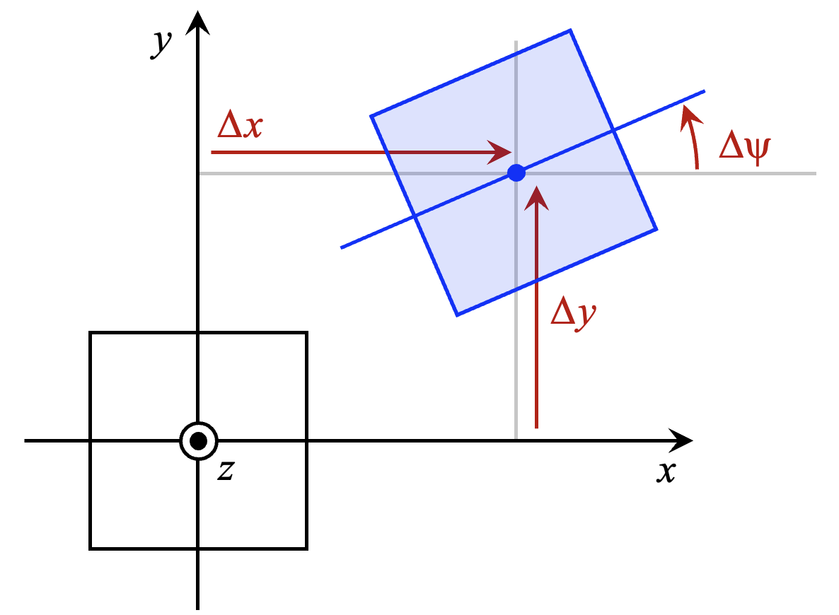
Misalignment in the the x-y plane.
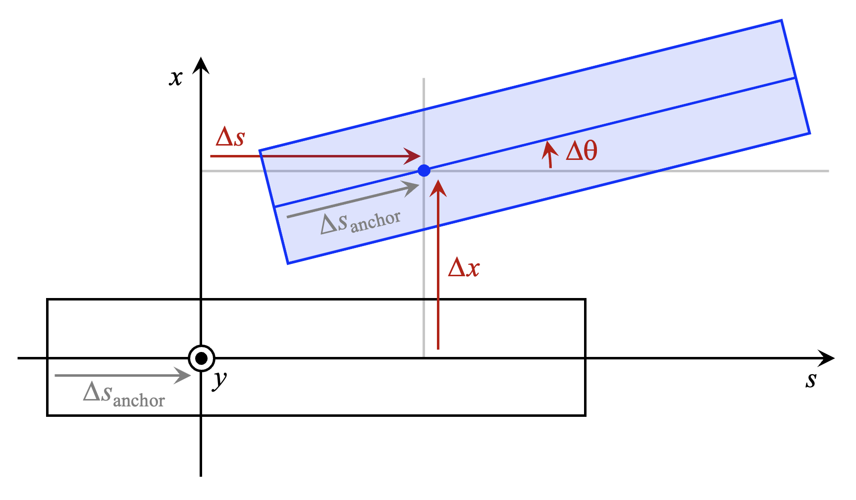
Misalignment in the the s-x plane.

Misalignment in the the s-y plane.
xtrack.Environment class
The Xsuite environment manages variables and elements that can be shared by different lines and can be used to create elements and line objects. See Xsuite environment in the User’s guide for tutorial examples.
Members - short description
Member |
Description |
|---|---|
Get the value of an expression |
|
Extend the order of the knl and ksl attributes of the elements. |
|
Extend the order of the rel_knl and rel_ksl attributes of the elements. |
|
Get an element or the value of a variable. |
|
Get expression associated to a variable |
|
Import a line into this environment. |
|
Get information about an element or a variable. |
|
Create a new element or line. |
|
Create a new expression |
|
Create a new line. |
|
Create a place object. |
|
Remove an element, particle, line, or variable by name. |
|
Replace a replica element with a clone of its parent element. Expressions on element attributes are preserved. |
|
Set the values or expressions of variables or element properties. A single call can set one or multiple variables or elements. |
|
Dictionary-like container of elements in the environment. |
|
xdeps reference container for element fields. |
|
Container of named beam elements stored in the environment. |
|
xdeps function container used in expressions. |
|
Names of all lines currently in the environment. |
|
Container of named lines registered in this environment. |
|
User metadata associated with the environment. |
|
xdeps reference container for variables, elements, particles, and lines. |
|
xdeps dependency manager for variables, element references, and expressions. |
|
Variables container associated with the environment. |
|
Xcoll-specific helpers associated with this environment. |
|
Xfields-specific helpers associated with this environment. |
Member |
Description |
|---|---|
Associate a particle type to a name. The particle is stored in Environment.particles, its properties can be controlled with deferred expressions and it can be used as reference particle for lines. |
|
Set the environment reference particle and optionally propagate it to lines. |
|
Reference particle associated with the environment. |
|
Container of named particle references stored in the environment. |
Member |
Description |
|---|---|
Change a set of knobs in the beam lines in order to match assigned targets. |
|
Match a new knob in the beam line such that the specified targets are matched when the knob is set to the value knob_value_end and the state of the line before tha matching is recovered when the knob is set to the value knob_value_start. |
|
Compute the twiss parameters for the lines. |
Member |
Description |
|---|---|
Build the trackers for the lines. |
|
Discard all trackers in all lines of the environment. |
Member |
Description |
|---|---|
Call a file with xtrack commands. |
|
Create a deep copy of the environment. |
|
Rebuild an environment from a serialized dictionary. |
|
Construct an environment from a JSON file. |
|
Serialize the environment to a JSON-compatible dictionary. |
|
Save the environment to a JSON file. |
Member |
Description |
|---|---|
Load a multiline from a MAD-X file. |
|
Deprecated. Create a new composer. |
|
Deprecated: set multipolar errors for specified elements of the environment. |
|
Convenience accessor to variable values. |
|
Short alias for variable values. |
Member |
Description |
|---|---|
Deprecated alias for |
|
Deprecated alias for |
|
Deprecated alias for |
Members - full description
Editing, Inspection, Variables and Configuration
Go to Summary table
- Environment.eval(expr)
Get the value of an expression
- Parameters:
expr (str) – Expression to evaluate.
- Returns:
value – Value of the expression.
- Return type:
float
Examples
import xtrack as xt

env = xt.Environment()
env['a'] = 2.0

value = env.eval('3*a + 1')

# value is 7.0
- Environment.extend_knl_ksl(order, element_names=None)
Extend the order of the knl and ksl attributes of the elements.
- Parameters:
order (int) – New order of the knl and ksl attributes.
element_names (list of str) – Names of the elements to extend. If None, all elements having knl and ksl attributes are extended.
- Environment.extend_knl_rel_ksl_rel(order, element_names=None)
Extend the order of the rel_knl and rel_ksl attributes of the elements.
- Parameters:
order (int) – New order of the rel_knl and rel_ksl attributes.
element_names (list of str) – Names of the elements to extend. If None, all elements having knl and ksl attributes are extended.
- Environment.get(key)
Get an element or the value of a variable.
- Parameters:
key (str) – Name of the element or variable.
- Returns:
element – Element or value of the variable.
- Return type:
Element or float
Examples
import xtrack as xt

env = xt.Environment()
env['kq'] = 0.2
env.new('qf', 'Quadrupole', length=1.0, k1='kq')

element = env.get('qf')
value = env.get('kq')

# element is the Quadrupole object; value is 0.2
- Environment.get_expr(var)
Get expression associated to a variable
- Parameters:
var (str) – Name of the variable
- Returns:
expr – Expression associated to the variable
- Return type:
Expression
Examples
import xtrack as xt

env = xt.Environment()
env['a'] = 2.0
env['b'] = '3*a'

expr = env.get_expr('b')

# expr is the expression controlling b.
# env.get_expr('a') returns None because a is a constant.
- Environment.import_line(line, suffix_for_common_elements=None, rename_elements={}, line_name=None, overwrite_vars=False)
Import a line into this environment.
- Parameters:
line (xtrack.Line) – Line to import. Its elements, variables, particle reference, configuration, and metadata are copied into this environment.
suffix_for_common_elements (str, optional) – Suffix to be added to the names of the elements that are common to the imported line and the line in this environment. If None,
'/{line_name}'is used.rename_elements (dict, optional) – Dictionary with the elements to be renamed. The keys are the names of the elements in
line, and the values are the new names.line_name (str, optional) – Name of the new line. If None, the name of the imported line is used.
overwrite_vars (bool, optional) – If True, the variables in the imported line will overwrite the variables with the same name in this environment. Default is False.
- Returns:
This method modifies the environment in place.
- Return type:
None
- Environment.info(key, limit=30)
Get information about an element or a variable.
- Parameters:
key (str) – Name of the element or variable.
limit (int, optional) – Maximum number of expression terms shown for variable info.
- Returns:
This method displays information and does not return a value.
- Return type:
None
Examples
import xtrack as xt

env = xt.Environment()
env['a'] = 2.0
env['kq'] = '3*a'
env.new('qf', 'Quadrupole', length=1.0, k1='kq')

env.info('kq')
# Info for vars['kq']
#
# value: 6.0
#
# controlled by expr:
#   vars['kq'] = (3.0 * vars['a'])
#
# expr_dependencies:
#   vars['a'] = 2.0
#
# controlled_targets:
#    element_refs['qf'].k1

env.info('qf')
# Element of type:  Quadrupole
# name                value   expr
# k1                  6.0     vars['kq']
# k1s                 0.0     None
# length              1.0     None
# ...
- Environment.new(name, prototype=None, mode=None, at=None, from_=None, anchor=None, from_anchor=None, extra=None, mirror=False, force=False, import_from=None, parent=None, **kwargs)
Create a new element or line.
- Parameters:
name (str) – Name of the new element or line
prototype (str or class) – Prototype class or name of the prototype element
parent (str or class, optional) – Deprecated alias for
prototype.mode (str, optional) –
clone: clone the prototype element or line. The prototype element or line is copied, together with the associated expressions.
replica: replicate the prototype elements or lines are made.
import: clone from a different environment. import_from must be provided.
at (float or str, optional) – Position of the created object.
from (str, optional) – Name of the element from which the position is calculated (its center is used as reference).
mirror (bool, optional) – Can only be used when cloning lines. If True, the order of the elements is reversed.
import_from (Environment, optional. Only to be used when mode is 'import'.) –
Notes
Environment.newcan instantiate only the built-in element classes supported by the line builder. For user-defined element classes, or other element types that are not supported byEnvironment.new, instantiate the element explicitly, store it inenv.elements, and attach deferred expressions through the environment view.- Returns:
Name of the created element or line or a Place object if at or from_ is provided.
- Return type:
str or Place
Examples
import xtrack as xt

env = xt.Environment()
env['kqf'] = 0.2
env.new('qf', 'Quadrupole', length=1.0, k1='kqf')
env.new('qd', 'qf', k1='-kqf')

env.ref['qd'].k1.xdeps.info()
# Info for element_refs['qd'].k1
#
# value: -0.2
#
# controlled by expr:
#   element_refs['qd'].k1 = (-vars['kqf'])
#
# expr_dependencies:
#   vars['kqf'] = 0.2
#
# controlled_targets: None
Unsupported or user-defined element classes can be added explicitly:
import xtrack as xt

class MyElement:
    def __init__(self, myparam=0):
        self.myparam = myparam

    def track(self, particles):
        pass

env = xt.Environment()
env['a'] = 2.0
env.elements['myelem'] = MyElement(myparam=0)
env['myelem'].myparam = '3*a'

env['myelem'].myparam
# 6.0
- Environment.new_expr(expr)
Create a new expression
- Parameters:
expr (str) – Expression to create.
- Returns:
expr – New expression.
- Return type:
Expression
Examples
import xtrack as xt

env = xt.Environment()
env['a'] = 2.0

expr = env.new_expr('3*a + 1')
env['b'] = expr

# env['b'] is 7.0
- Environment.new_line(components=None, name=None, refer: Literal['start', 'center', 'centre', 'end'] = 'center', length=None, mirror=False, s_tol=1e-06, compose=False) Line
Create a new line.
- Parameters:
components (list, optional) – List of components to be added to the line. It can include strings, place objects, and lines.
name (str, optional) – Name of the new line.
refer (str, optional) – Specifies which part of the component the
atposition will refer to. Allowed values arestart,center(default; also allowed iscentre), andend.length (float | str, optional) – Length of the line to be built by the composer. Can be an expression. If not specified, the length will be the minimum length that can fit all the components.
mirror (bool, optional) – Whether the line should be mirrored after creation.
compose (bool, optional) – Whether to instantiate the line in
composemode, which allows the components to be added to the line after creation.s_tol (float, optional) – Difference between two s positions below which they should be treated as the same location.
- Returns:
The new line.
- Return type:
line
Examples
import xtrack as xt

env = xt.Environment()
env['a'] = 3 # Define a variable
env.new('mq1', 'Quadrupole', length=0.3, k1='a')
env.new('mq2', 'Quadrupole', length=0.3, k1='-a')

ln = env.new_line(name='myline', components=[
    'mq1',
    env.new('mymark', 'Marker', at=10.0),
    env.new('mq1_clone', 'mq1', k1='2*a'),
    env.place('mq2', at=20.0, from_='mymark'),
])
- Environment.place(name, obj=None, at=None, from_=None, anchor=None, from_anchor=None)
Create a place object.
- Parameters:
name (str or Line) – Name of the element or line to be placed.
at (float or str, optional) – Position of the created object.
from (str, optional) – Name of the element from which the position is calculated (its center is used as reference).
- Returns:
The new place object.
- Return type:
Place
Examples
import xtrack as xt

env = xt.Environment()
env.new('qf', 'Quadrupole', length=2.0)
env.new('mk', 'Marker')

line = env.new_line(components=[
    env.place('qf', at=3.0),
])

line.insert([
    env.place('mk', at=0, from_='qf', from_anchor='center'),
])

line.get_table().show()
# name                      s element_type             isthick ...
# ||drift_1                 0 Drift                       True
# qf_entry                  2 Marker                     False
# qf..entry_map             2 ThinSliceQuadrupoleEntry   False
# qf..0                     2 ThickSliceQuadrupole        True
# mk                        3 Marker                     False
# qf..1                     3 ThickSliceQuadrupole        True
# qf..exit_map              4 ThinSliceQuadrupoleExit    False
# qf_exit                   4 Marker                     False
# _end_point                4                            False
- Environment.remove(key)
Remove an element, particle, line, or variable by name.
- Parameters:
key (str) – Name of the object to remove.
Examples
import xtrack as xt

env = xt.Environment()
env.new('qf', 'Quadrupole', length=1.0)

env.remove('qf')

# 'qf' is no longer in env
- Environment.replace_replica(name)
Replace a replica element with a clone of its parent element. Expressions on element attributes are preserved.
- Parameters:
name (str) – Name of the replica element to replace.
- Returns:
This method modifies the environment in place.
- Return type:
None
- Environment.set(name, *args, **kwargs)
Set the values or expressions of variables or element properties. A single call can set one or multiple variables or elements.
- Parameters:
name (str or iterable of str) – Name or names of the variable(s) or element(s).
value (float or str) – Value or expression of the variable to set. Can be provided only if the name is associated to a variable.
**kwargs – Attributes to set. Can be provided only if the name is associated to an element.
str (float or) – Attributes to set. Can be provided only if the name is associated to an element.
Examples
>>> line.set('a', 0.1)
>>> line.set('k1', '3*a')
>>> line.set('quad', k1=0.1, k2='3*a')
>>> line.set(['quad1', 'quad2'], k1=0.1, k2='3*a')
>>> line.set(['c', 'd'], 0.1)
>>> line.set(['e', 'f'], '3*a')
- property Environment.element_dict
Dictionary-like container of elements in the environment.
- Returns:
element_dict – Mapping from element names to element objects.
- Return type:
dict
- property Environment.element_refs
xdeps reference container for element fields.
- Returns:
element_refs – Dictionary-like container of xdeps element references, or
Nonewhen variable management is disabled.- Return type:
object
- property Environment.elements
Container of named beam elements stored in the environment.
Use this container to inspect, add, replace, or remove elements by name. Element names share the environment namespace with variables, particles, and lines.
- Returns:
elements – Dictionary-like container of elements. When expression management is enabled, item access returns reference-aware views.
- Return type:
Examples
import xtrack as xt

env = xt.Environment()
env.elements['qf'] = xt.Quadrupole(length=1.0, k1=0.2)

env.elements.get_table().show()
# name element_type isthick isreplica parent_name ... length
# qf   Quadrupole      True     False None        ...      1
- property Environment.functions
xdeps function container used in expressions.
- Returns:
functions – Dictionary-like container of functions available in expressions.
- Return type:
object
Examples
import xtrack as xt

env = xt.Environment()
env['t_turn_s'] = 0.5
env.functions['ramp'] = xt.FunctionPieceWiseLinear(
    x=[0, 1], y=[0.2, 0.4])
env['kq'] = env.functions['ramp'](env.ref['t_turn_s'])

env.ref['kq'].xdeps.info()
# Info for vars['kq']
#
# value: 0.30000000000000004
#
# controlled by expr:
#   vars['kq'] = f['ramp'](vars['t_turn_s'])
#
# expr_dependencies:
#   f['ramp'] = <xdeps.functions.FunctionPieceWiseLinear object at ...>
#   vars['t_turn_s'] = 0.5
- property Environment.line_names
Names of all lines currently in the environment.
- Returns:
line_names – Line names in insertion order.
- Return type:
list of str
- property Environment.lines
Container of named lines registered in this environment.
- Returns:
lines – Dictionary-like container exposing lines by name.
- Return type:
Examples
import xtrack as xt

env = xt.Environment()
env.new('qf', 'Quadrupole', length=1.0)
env.new('qd', 'Quadrupole', length=1.0)
env.new('ip', 'Marker')

env.new_line(name='cell', components=[
    env.place('ip', at=0.0),
    env.place('qf', at=2.0, from_='ip'),
    env.place('qd', at=4.0, from_='qf'),
])

env.lines['cell'].get_table().show()
# name                   s element_type isthick ...
# ip                     0 Marker         False
# ||drift_1              0 Drift           True
# qf                   1.5 Quadrupole      True
# ||drift_2            2.5 Drift           True
# qd                   5.5 Quadrupole      True
# _end_point           6.5                False
- property Environment.metadata
User metadata associated with the environment.
- Returns:
metadata – Mutable dictionary storing user metadata.
- Return type:
dict
- property Environment.ref
xdeps reference container for variables, elements, particles, and lines.
References can be used to build deferred expressions that stay linked to the underlying environment quantities.
- Returns:
ref – Reference container for environment objects.
- Return type:
Examples
import xtrack as xt

env = xt.Environment()
env['kq'] = 0.2
env.new('qf', 'Quadrupole', length=1.0)
env.ref['qf'].k1 = 2 * env.ref['kq']

env.ref['qf'].k1.xdeps.info()
# Info for element_refs['qf'].k1
#
# value: 0.4
#
# controlled by expr:
#   element_refs['qf'].k1 = (2 * vars['kq'])
- property Environment.ref_manager
xdeps dependency manager for variables, element references, and expressions.
- Returns:
ref_manager – Dependency manager used to register and update expression tasks.
- Return type:
object
- property Environment.vars
Variables container associated with the environment.
The container provides variable-management utilities such as
keys(),get_table(),load()(JSON and MAD-X files),remove(),rename(), andupdate().- Returns:
vars – Dictionary-like container of variables.
- Return type:
Examples
import xtrack as xt

env = xt.Environment()
env.vars['a'] = 2.0
env.vars['b'] = '3*a'

env.vars.get_table().show()
# name       value expr
# t_turn_s       0 None
# a              2 None
# b              6 (3.0 * a)
- property Environment.xcoll
Xcoll-specific helpers associated with this environment.
- Returns:
xcoll – Accessor exposing Xcoll helper methods.
- Return type:
xcoll.environment_tools.XcollEnvironmentAPI
- property Environment.xfields
Xfields-specific helpers associated with this environment.
- Returns:
xfields – Accessor exposing Xfields helper methods.
- Return type:
Reference Particle and Particle Generation
Go to Summary table
- Environment.new_particle(name, parent=None, force=False, **kwargs)
Associate a particle type to a name. The particle is stored in Environment.particles, its properties can be controlled with deferred expressions and it can be used as reference particle for lines.
Note that this method is not meant to create particles distributions for tracking. For that purpose use xt.Particles(…), Line.build_particles(…) or the generation functions for particles distributions available in xpart. See https://xsuite.readthedocs.io/en/latest/particlesmanip.html for more details.
- Parameters:
name (str) – Name of the new particle type
parent (str or class) – Parent class or name of the parent particle type
pdg_id_0 (int or str, optional, define reference mass and charge from) – PDG id or particle name.
mass0 (float, optional) – Reference rest mass [eV]
q0 (float, optional) – Reference charge [e]
p0c (array_like of float, optional) – Reference momentum [eV]
energy0 (array_like of float, optional) – Reference energy [eV]
gamma0 (array_like of float, optional) – Reference relativistic gamma
beta0 (array_like of float, optional) – Reference relativistic beta
rigidity0 (array_like of float, optional) – Reference magnetic rigidity [T.m]
kinetic_energy0 (array_like of float, optional) – Reference kinetic energy [eV]
Examples
Create a positron particle type with gamma0 controlled by a deferred expression:
>>> env = xt.Environment()
>>> env['a'] = 5
>>> env.new_particle('my_particle_type', pdg_id_0='positron', gamma0='3*a')
'my_particle_type'
>>> env['my_particle_type'].gamma0
View of LinkedArrayCpu([15.])
>>> env['a'] = 10
>>> env['my_particle_type'].gamma0
View of LinkedArrayCpu([30.])
- Environment.set_particle_ref(*args, lines=True, **kwargs)
Set the environment reference particle and optionally propagate it to lines.
- Parameters:
*args – Either a single
xtrack.Particles, a particle name, or arguments passed toxtrack.Particles.lines (bool, str, iterable of str, optional) – Which lines receive the same reference particle.
Trueupdates all lines,False/Noneupdates none.**kwargs – Extra keyword arguments forwarded to
xtrack.Particleswhen constructing a new particle reference.
- property Environment.particle_ref
Reference particle associated with the environment.
- Returns:
particle_ref – Proxy to the configured reference particle, or
Nonewhen no reference particle is configured.- Return type:
- property Environment.particles
Container of named particle references stored in the environment.
Named particles can be used as reusable reference particles for lines or accessed directly through the environment.
- Returns:
particles – Dictionary-like container of particles. When expression management is enabled, item access returns reference-aware views.
- Return type:
Examples
import xtrack as xt

env = xt.Environment()
env['pc'] = 7e12
env.new_particle('lhc_proton', 'proton', p0c='pc')

env.particles.get_table().show()
# name          mass0 charge0 energy0   p0c gamma0 beta0
# lhc_proton 9.38272e+08   1   7e+12 7e+12 7460.52     1
Analysis and Matching
Go to Summary table
- Environment.match(vary, targets, restore_if_fail=True, solver=None, verbose=False, check_limits=True, **kwargs)
Change a set of knobs in the beam lines in order to match assigned targets.
- Parameters:
vary (list of str or list of Vary objects) – List of knobs to be varied. Each knob can be a string or a Vary object including the knob name and the step used for computing the Jacobian for the optimization.
targets (list of Target objects) – List of targets to be matched.
restore_if_fail (bool) – If True, the beamline is restored to its initial state if the matching fails.
solver (str) – Solver to be used for the matching.
check_limits (bool) – If True (default), the limits of the knobs are checked before the optimization. If False, if the knobs are out of limits, the optimization knobs are set to the limits on the first iteration.
verbose (bool) – If True, the matching steps are printed.
**kwargs (dict) – Additional arguments to be passed to the twiss.
- Returns:
result_info – Dictionary containing information about the matching result.
- Return type:
dict
- Environment.match_knob(knob_name, vary, targets, knob_value_start=0, knob_value_end=1, **kwargs)
Match a new knob in the beam line such that the specified targets are matched when the knob is set to the value knob_value_end and the state of the line before tha matching is recovered when the knob is set to the value knob_value_start.
- Parameters:
knob_name (str) – Name of the knob to be matched.
vary (list of str or list of Vary objects) – List of existing knobs to be varied.
targets (list of Target objects) – List of targets to be matched.
knob_value_start (float) – Value of the knob before the matching. Defaults to 0.
knob_value_end (float) – Value of the knob after the matching. Defaults to 1.
- Environment.twiss(lines=None, **kwargs)
Compute the twiss parameters for the lines.
- Parameters:
lines (list of str) – The lines for which the twiss parameters are computed. If None, the twiss parameters are computed for all lines.
**kwargs (dict) – Additional keyword arguments are passed to the Line.twiss method.
- Returns:
out – A MultiTwiss object containing the twiss parameters for the lines.
- Return type:
MultiTwiss
Tracker Setup
Go to Summary table
- Environment.build_trackers(_context=None, _buffer=None, **kwargs)
Build the trackers for the lines.
- Parameters:
_context (xobjects.Context) – The context in which the trackers are built.
_buffer (xobjects.Buffer) – The buffer in which the trackers are built.
**kwargs (dict) – Additional keyword arguments are passed to the Line.build_tracker method.
- Environment.discard_trackers()
Discard all trackers in all lines of the environment.
- Returns:
This method modifies the environment lines in place.
- Return type:
None
Constructors and Serialization
Go to Summary table
- Environment.call(filename)
Call a file with xtrack commands.
- Parameters:
filename (str) – Name of the file to be called.
- Environment.copy()
Create a deep copy of the environment.
- Returns:
Independent copy of the environment, including elements, lines, particles, variables, expressions and metadata.
- Return type:
Environment
- classmethod Environment.from_dict(dct, _context=None, _buffer=None, classes=())
Rebuild an environment from a serialized dictionary.
- Parameters:
dct (dict) – Dictionary produced by
to_dict()._context (xobjects.Context, optional) – Context used to rebuild xobjects-backed data.
_buffer (xobjects.Buffer, optional) – Buffer used to rebuild xobjects-backed data.
classes (tuple, optional) – Extra element classes accepted during element deserialization.
- Returns:
Reconstructed environment.
- Return type:
Environment
- classmethod Environment.from_json(file, **kwargs)
Construct an environment from a JSON file.
- Parameters:
file (str or file-like object) – Path to the JSON file or file-like object. If the filename ends with
.gz, the file is decompressed.**kwargs (dict) – Additional keyword arguments passed to
Environment.from_dict.
- Returns:
environment – Environment object.
- Return type:
Environment
- Environment.to_dict(include_var_management=True, include_version=True)
Serialize the environment to a JSON-compatible dictionary.
- Parameters:
include_var_management (bool, optional) – If True, include deferred-expression data and variable manager state. Default is
True.include_version (bool, optional) – If True, include the xtrack version that generated the dictionary. Default is
True.
- Returns:
Serialized environment data.
- Return type:
dict
- Environment.to_json(file, indent=1, **kwargs)
Save the environment to a JSON file.
- Parameters:
file (str or file-like object) – The file to save to. If a string is provided, a file is opened and closed. If a file-like object is provided, it is used directly.
indent (int, optional) – Indentation level used for the JSON output. Default is 1.
**kwargs – Additional keyword arguments passed to
Environment.to_dict.
- Returns:
This method writes the serialized environment to
file.- Return type:
None
Deprecated
Go to Summary table
- classmethod Environment.from_madx(filename=None, madx=None, stdout=None, return_lines=False, **kwargs)
Load a multiline from a MAD-X file.
Warning
This function is deprecated and will be removed in a future version. Please use xtrack.load(…), which uses the xsuite native MAD-X parser, without requiring Cpymad. In case you need to use cpymad for specific features, please load the individual lines using Line.from_madx_sequence(…) and add them to the environment using Environment.import_line(…).
- Parameters:
filename (str, optional) – The MAD-X file to load from.
madx (cpymad.madx.Madx, optional) – Existing MAD-X instance to load from.
stdout (object, optional) – Stream used by the legacy MAD-X loader.
return_lines (bool, optional) – Whether to return individual lines instead of an environment.
**kwargs – Additional keyword arguments are passed to the
Line.from_madx_sequencemethod.
- Returns:
new_multiline – The multiline object.
- Return type:
Multiline
- Environment.new_builder(components=None, name=None, refer: Literal['start', 'center', 'centre', 'end'] = 'center', length=None, s_tol=1e-06)
Deprecated. Create a new composer.
Warning
The new_builder method is deprecated and will be removed in a future version. Use new_line with compose=True instead.
- Parameters:
components (list, optional) – List of components to be added to the composer. It can include strings, place objects, and lines.
name (str, optional) – Name of the line that will be built by the composer.
refer (str, optional) – Specifies which part of the component the
atposition will refer to. Allowed values arestart,center(default; also allowed iscentre), andend.length (float | str, optional) – Length of the line to be built by the composer. Can be an expression. If not specified, the length will be the minimum length that can fit all the components.
- Returns:
The new composer.
- Return type:
Composer
- Environment.set_multipolar_errors(errors)
Deprecated: set multipolar errors for specified elements of the environment.
Warning
This function is deprecated and will be removed in a future version. Please use the attributes knl_rel and ksl_rel of the elements to set relative multipolar errors directly on the elements.
- Parameters:
errors (dict) –
Dictionary with the errors to be set. The keys are the names of the elements, and the values are dictionaries with the following keys:
rel_knl: list of relative errors for the normal multipolar strengths.
rel_ksl: list of relative errors for the skew multipolar strengths.
refer: name of the strength to be used as reference, which is multiplied by the length. If None, the default reference strength is used (k0 for bends, k1 for quadrupoles, k2 for sextupoles, and k3 for octupoles).
Examples
env = xt.Environment()
env.vars.default_to_zero = True
line = env.new_line(components=[
    env.new('mq', 'Quadrupole', length=0.5, k1='kq'),
    env.new('mqs', 'Quadrupole', length=0.5, k1s='kqs'),
    env.new('mb', 'Bend', length=0.5, angle='ang', k0_from_h=True),
])

env.set_multipolar_errors({
    'mq': {'rel_knl': [1e-6, 1e-5, 1e-4],
           'rel_ksl': [-1e-6, -1e-5, -1e-4]},
    'mqs': {'rel_knl': [2e-6, 2e-5, 2e-4],
            'rel_ksl': [3e-6, 3e-5, 3e-4],
            'refer': 'k1s'},
    'mb': {'rel_knl': [2e-6, 3e-5, 4e-4],
           'rel_ksl': [5e-6, 6e-5, 7e-4]},
    })
- property Environment.varval
Convenience accessor to variable values.
Warning
Environment.varval[...]is deprecated and will be removed in a future version. To access the value of a variable you can simply useEnvironment[...].Equivalent to
environment.vars.val.- Returns:
values – Mapping-like view exposing variable values.
- Return type:
object
- property Environment.vv
Short alias for variable values.
Warning
Environment.vv[...]is deprecated and will be removed in a future version. To access the value of a variable you can simply useEnvironment[...].Equivalent to
environment.varval(orenvironment.vars.val).- Returns:
values – Mapping-like view exposing variable values.
- Return type:
object
Upcoming deprecations
Go to Summary table
- Environment.apply_filling_pattern(filling_pattern_cw, filling_pattern_acw, i_bunch_cw, i_bunch_acw)
Deprecated alias for
env.xfields.apply_filling_pattern(...).Warning
This method is deprecated and will be removed in a future version. Use
env.xfields.apply_filling_pattern(...)instead.- Parameters:
filling_pattern_cw (array_like) – Filling pattern for the clockwise beam.
filling_pattern_acw (array_like) – Filling pattern for the anticlockwise beam.
i_bunch_cw (int) – Bunch index for the clockwise beam.
i_bunch_acw (int) – Bunch index for the anticlockwise beam.
- Returns:
Result returned by
env.xfields.apply_filling_pattern(...).- Return type:
object
- Environment.configure_beambeam_interactions(num_particles, nemitt_x, nemitt_y, crab_strong_beam=True, use_antisymmetry=False, separation_bumps=None)
Deprecated alias for
env.xfields.configure_beambeam_interactions(...).Warning
This method is deprecated and will be removed in a future version. Use
env.xfields.configure_beambeam_interactions(...)instead.- Parameters:
num_particles (float) – Number of particles per bunch.
nemitt_x (float) – Horizontal normalized emittance.
nemitt_y (float) – Vertical normalized emittance.
crab_strong_beam (bool, optional) – Whether to include strong-beam crabbing.
use_antisymmetry (bool, optional) – Whether to use antisymmetry when configuring the interactions.
separation_bumps (object, optional) – Separation bump configuration passed to the Xfields helper.
- Returns:
Result returned by
env.xfields.configure_beambeam_interactions(...).- Return type:
object
- Environment.install_beambeam_interactions(clockwise_line, anticlockwise_line, ip_names, num_long_range_encounters_per_side, num_slices_head_on, harmonic_number, bunch_spacing_buckets, sigmaz, delay_at_ips_slots=None)
Deprecated alias for
env.xfields.install_beambeam_interactions(...).Warning
This method is deprecated and will be removed in a future version. Use
env.xfields.install_beambeam_interactions(...)instead.- Parameters:
clockwise_line (str or xtrack.Line) – Clockwise line or line name.
anticlockwise_line (str or xtrack.Line) – Anticlockwise line or line name.
ip_names (sequence of str) – Interaction point names.
num_long_range_encounters_per_side (int or sequence of int) – Number of long-range encounters per side.
num_slices_head_on (int) – Number of longitudinal slices for head-on interactions.
harmonic_number (int) – RF harmonic number.
bunch_spacing_buckets (int) – Bunch spacing in RF buckets.
sigmaz (float) – RMS bunch length.
delay_at_ips_slots (sequence of int, optional) – Delay at interaction points in bunch slots.
- Returns:
Result returned by
env.xfields.install_beambeam_interactions(...).- Return type:
object
Environment containers
- class xtrack.environment.EnvVars(env)
Container for variables stored in an environment.
Instances are available as
env.varsand provide dictionary-like access to environment variables, expressions, variable values, and variable table generation.- keys()
Return the variable names in the environment.
- Returns:
Variable names, including internal variables.
- Return type:
list of str
- update(*args, **kwargs)
Update environment variables.
Variables can be supplied as a mapping positional argument and/or as keyword arguments. String values are interpreted as expressions.
- Parameters:
*args – Optional single mapping of variable names to values or expressions.
default_to_zero (bool, optional) – Temporarily set whether missing variables default to zero while applying the update.
**kwargs – Variable names and values or expressions to set.
- load(file=None, string=None, format: Literal['json', 'madx', 'python'] = None, timeout=5.0)
Load variables from a file or string.
- Parameters:
file (str or pathlib.Path, optional) – File path or URL to load. Supported formats are JSON, MAD-X, and Python files.
string (str, optional) – Source string to load. The
formatargument must be provided when loading from a string.format ({"json", "madx", "python"}, optional) – Input format. If omitted for files, it is inferred from the file extension when possible.
timeout (float, optional) – Timeout in seconds used when reading from a URL.
- Returns:
Environment loaded from a Python file, or
Nonefor JSON and MAD-X inputs.- Return type:
xtrack.Environment or None
- property vary_default
Default vary settings stored in the environment.
- Returns:
Dictionary with default vary settings.
- Return type:
dict
- get_table(compact=True, expr_obj=False)
Return a table with environment variables.
- Parameters:
compact (bool, optional) – If
True, format expressions using compact names.expr_obj (bool, optional) – If
True, include anexpr_objcolumn with expression objects.
- Returns:
Table with variable names, values, and expressions.
- Return type:
- new_expr(expr)
Build an expression from a string.
- Parameters:
expr (str) – Expression to evaluate in the environment expression context.
- Returns:
xdeps expression or value resulting from the evaluation.
- Return type:
object
- eval(expr)
Evaluate an expression or variable reference.
- Parameters:
expr (str) – Expression to evaluate in the environment expression context.
- Returns:
Numerical value if the expression evaluates to a reference, otherwise the evaluated expression object or value.
- Return type:
object
- info(var, limit=10)
Return dependency information for a variable.
- Parameters:
var (str) – Variable name.
limit (int, optional) – Maximum number of dependencies to display.
- Returns:
Information returned by xdeps for the selected variable.
- Return type:
object
- get_expr(var)
Return the expression associated with a variable.
- Parameters:
var (str) – Variable name.
- Returns:
Expression associated with the variable, or
Nonefor an independent variable.- Return type:
object
- rename(old, new, verbose=False)
Rename a variable and update dependent expressions.
- Parameters:
old (str) – Current variable name.
new (str) – New variable name.
verbose (bool, optional) – If
True, print information about updated dependencies.
- get_independent_vars()
Return independent variables in the environment.
- Returns:
Names of variables that are not defined by expressions.
- Return type:
list of str
- load_madx(filename=None, string=None)
Load variables from MAD-X input.
Warning
This method is deprecated. Use
load()instead.- Parameters:
filename (str, optional) – Path to the MAD-X file to load.
string (str, optional) – MAD-X source string to load.
- set_from_madx_file(filename=None, string=None)
Load variables from MAD-X input.
Warning
This method is deprecated. Use
load()instead.- Parameters:
filename (str, optional) – Path to the MAD-X file to load.
string (str, optional) – MAD-X source string to load.
- load_madx_optics_file(filename=None, string=None)
Load variables from a MAD-X optics file.
Warning
This method is deprecated. Use
load()instead.- Parameters:
filename (str, optional) – Path to the MAD-X optics file to load.
string (str, optional) – MAD-X source string to load.
- load_json(filename)
Load variables from a JSON file.
Warning
This method is deprecated. Use
load()instead.- Parameters:
filename (str) – Path to the JSON file to load.
- target(tar, value, **kwargs)
Build a matching target for an environment variable.
- Parameters:
tar (str) – Variable name to target.
value (float or object) – Target value or constraint.
**kwargs – Additional keyword arguments passed to
xtrack.Target.
- Returns:
Target acting on environment variables.
- Return type:
- set(name, value)
Set a variable value or expression.
- Parameters:
name (str) – Variable name.
value (float or str or object) – Value to assign. Strings are interpreted as expressions.
- get(name)
Return the current value of a variable.
- Parameters:
name (str) – Variable name.
- Returns:
Current variable value.
- Return type:
object
- property default_to_zero
Whether missing variables default to zero.
- Returns:
Trueif missing variables default to zero, otherwiseFalse.- Return type:
bool
- remove(name)
Remove a variable from the environment.
- Parameters:
name (str) – Variable name to remove.
- Raises:
KeyError – If no variable with the requested name is present.
- class xtrack.environment.EnvElements(env)
Container for elements stored in an environment.
Instances are available as
env.elements. The container provides dictionary-like access to named elements and returns reference-aware views when the environment has variable management enabled.- get_table(attr=False)
Return a table with the elements stored in the environment.
- Parameters:
attr (bool, optional) – If
True, include element attribute columns.- Returns:
Table containing one row per environment element.
- Return type:
- remove(name)
Remove an element from the environment.
- Parameters:
name (str) – Name of the element to remove.
- Raises:
KeyError – If no element with the requested name is present.
- class xtrack.environment.EnvParticles(env)
Container for named particle references stored in an environment.
Instances are available as
env.particles. The container provides dictionary-like access to particle objects and returns reference-aware views when the environment has variable management enabled.- get_table()
Return a table with the particle references stored in the environment.
- Returns:
Table containing one row per particle reference, with mass, charge, energy, momentum, gamma, and beta columns.
- Return type:
- remove(name)
Remove a particle reference from the environment.
- Parameters:
name (str) – Name of the particle reference to remove.
- Raises:
KeyError – If no particle reference with the requested name is present.
- class xtrack.environment.EnvLines(env)
Container for lines stored in an environment.
Instances are available as
env.linesand provide dictionary-like access to namedxtrack.Lineobjects.- get_table()
Return a table with the lines stored in the environment.
- Returns:
Table containing one row per line, with line name, number of elements, and mode.
- Return type:
- remove(name)
Remove a line from the environment.
- Parameters:
name (str) – Name of the line to remove.
- class xtrack.environment.EnvRef(env)
Reference container for environment objects.
Instances are available as
env.refand provide access to xdeps references for variables, elements, particle references, and lines.- property elements
xdeps reference container for environment elements.
- Returns:
Reference container for element fields.
- Return type:
xdeps.refs.Ref
- property particles
xdeps reference container for environment particle references.
- Returns:
Reference container for particle reference fields.
- Return type:
xdeps.refs.Ref
- property vars
xdeps reference container for environment variables.
- Returns:
Reference container for variables.
- Return type:
xdeps.refs.Ref
- class xtrack.environment.EnvParticleRef(env)
Proxy for the environment reference particle.
Instances are used internally by
xtrack.Environmentto expose the current reference particle while allowing the reference particle to be stored either directly or by name.- copy(**kwargs)
Copy the resolved reference particle.
- Parameters:
**kwargs – Keyword arguments passed to the particle
copymethod.- Returns:
Copy of the resolved reference particle.
- Return type:
xpart.Particles
- class xtrack.environment.EnvXfields(env)
Accessor for Xfields-related environment helpers.
Instances are available as
env.xfieldsand expose helpers for beam-beam configuration workflows.- install_beambeam_interactions(clockwise_line, anticlockwise_line, ip_names, num_long_range_encounters_per_side, num_slices_head_on, harmonic_number, bunch_spacing_buckets, sigmaz, delay_at_ips_slots=None)
Install beam-beam interactions in two lines.
- Parameters:
clockwise_line (str or xtrack.Line) – Clockwise line or line name.
anticlockwise_line (str or xtrack.Line) – Anticlockwise line or line name.
ip_names (sequence of str) – Interaction point names.
num_long_range_encounters_per_side (int or sequence of int) – Number of long-range encounters per side.
num_slices_head_on (int) – Number of longitudinal slices for head-on interactions.
harmonic_number (int) – RF harmonic number.
bunch_spacing_buckets (int) – Bunch spacing in RF buckets.
sigmaz (float) – RMS bunch length.
delay_at_ips_slots (sequence of int, optional) – Delay at interaction points in bunch slots.
- Returns:
Result returned by the underlying beam-beam installation helper.
- Return type:
object
- configure_beambeam_interactions(num_particles, nemitt_x, nemitt_y, crab_strong_beam=True, use_antisymmetry=False, separation_bumps=None)
Configure installed beam-beam interactions.
- Parameters:
num_particles (float) – Number of particles per bunch.
nemitt_x (float) – Horizontal normalized emittance.
nemitt_y (float) – Vertical normalized emittance.
crab_strong_beam (bool, optional) – Whether to include strong-beam crabbing.
use_antisymmetry (bool, optional) – Whether to use antisymmetry when configuring the interactions.
separation_bumps (object, optional) – Separation bump configuration passed to the underlying helper.
- Returns:
Result returned by the underlying beam-beam configuration helper.
- Return type:
object
- apply_filling_pattern(filling_pattern_cw, filling_pattern_acw, i_bunch_cw, i_bunch_acw)
Apply filling patterns to the configured beam-beam interactions.
- Parameters:
filling_pattern_cw (array_like) – Filling pattern for the clockwise beam.
filling_pattern_acw (array_like) – Filling pattern for the anticlockwise beam.
i_bunch_cw (int) – Bunch index for the clockwise beam.
i_bunch_acw (int) – Bunch index for the anticlockwise beam.
- Returns:
Result returned by the underlying filling-pattern helper.
- Return type:
object
VarsTable
The xtrack.environment.VarsTable class is the table returned by
environment variable table methods such as env.vars.get_table().
See Working with tables in the User’s guide for an overview of the features offered by Table objects.
- class xtrack.environment.VarsTable(data, *args, **kwargs)
Table returned by environment variable table methods.
VarsTablestores one row per environment variable. The main columns are the variable name, its current value, and the expression that defines it, when present. It is returned by methods such asenv.vars.get_table().Create a variable table.
- Parameters:
data (mapping) – Mapping containing variable-table columns. Typical columns are
name,value, andexpr.*args – Additional positional arguments passed to
xtrack.Table.**kwargs – Additional keyword arguments passed to
xtrack.Table.
Examples
Build a small variable table:
>>> import numpy as np
>>> from xtrack.environment import VarsTable
>>> tab = VarsTable({
...     "name": np.array(["kqf", "kqd", "on_rf"], dtype=object),
...     "value": np.array([0.12, -0.12, 1.0]),
...     "expr": np.array([None, "-kqf", None], dtype=object),
... })
>>> tab
VarsTable: 3 rows, 3 cols
name          value expr
kqf            0.12 None
kqd           -0.12 -kqf
on_rf             1 None
Select variables by name pattern:
>>> tab.rows.match(name="kq.*")
VarsTable: 2 rows, 3 cols
name         value expr
kqf           0.12 None
kqd          -0.12 -kqf
- property cols
Access column-selection helpers.
The returned view is used to select multiple columns while preserving the table type. Columns can be selected from a whitespace-separated string or from an iterable of column names. String selectors can also contain simple expressions involving table columns, for example
"dx/sqrt(betx)".- Returns:
Accessor exposing column selection and column utilities.
- Return type:
Examples
Select a subset of columns:
>>> table.cols["betx bety alfx alfy"]
Select columns together with an expression:
>>> table.cols["betx dx dx/sqrt(betx)"]
Column selections return table objects and can be chained with row selections:
>>> table.rows.match(element_type="Quadrupole").cols["s betx bety"]
- classmethod concatenate(tables)
Concatenate a list of tables.
- Parameters:
tables (sequence of xdeps.Table) – Tables to concatenate. Only columns present in all tables are kept.
- Returns:
Concatenated table.
- Return type:
xdeps.Table
- classmethod from_csv(file)
Reconstruct a table instance from CSV data.
- Parameters:
file (str or path-like or file-like) – CSV file or file-like object to read.
- Returns:
Reconstructed table.
- Return type:
- classmethod from_dict(dct: Dict[str, Any])
Construct a table from its dictionary representation.
- Parameters:
dct (dict) – Dictionary produced by
to_dict().- Returns:
Reconstructed table.
- Return type:
- classmethod from_hdf5(file, *, group=None)
Load a table from an HDF5 file or group.
- Parameters:
file (str or path-like or file-like or h5py.File or h5py.Group) – HDF5 input target.
group (str or None, optional) – HDF5 group containing the serialized table. If
None, the file must contain exactly one group.
- Returns:
Reconstructed table.
- Return type:
- classmethod from_json(file)
Load a serialized table from JSON.
- Parameters:
file (str or path-like or file-like) – JSON file or file-like object to read.
- Returns:
Reconstructed table.
- Return type:
- classmethod from_pandas(df, index=None, lowercase=False)
Build a table from a pandas DataFrame.
- Parameters:
df (pandas.DataFrame) – DataFrame containing the table data.
index (str or None, optional) – Column to use as the table index. If
None, use the DataFrame index name when available, or"NAME"if present.lowercase (bool, optional) – If
True, lowercase column names, string columns, and string headers before building the table.
- Returns:
Table built from the DataFrame.
- Return type:
xdeps.Table
- classmethod from_rows(rows, col_names=None, index=None)
Build a table from row objects.
- Parameters:
rows (sequence of mapping, namedtuple, or dataclass instances) – Row data used to populate the table.
col_names (sequence of str or None, optional) – Columns to include. If
None, infer columns from the first row.index (str or None, optional) – Column to use as the table index.
- Returns:
Table built from the supplied rows.
- Return type:
xdeps.Table
- classmethod from_tfs(file)
Load a table from a TFS file.
- Parameters:
file (str or path-like or file-like) – TFS input source.
- Returns:
Reconstructed table.
- Return type:
- items()
Return an iterator over table data items.
- Returns:
View over
(name, value)pairs in the underlying table data.- Return type:
dict_items
- keys(exclude_columns=False)
Return table data keys.
- Parameters:
exclude_columns (bool, optional) – If
True, return only data keys that are not table columns.- Returns:
Underlying data keys, or a set of non-column data keys when
exclude_columnsisTrue.- Return type:
dict_keys or set
- property mask
Deprecated row-mask accessor.
- Raises:
DeprecationWarning – Always raised. Use
table.rows.maskortable.rows.indicesinstead.
- pop(key)
Remove and return a table data entry.
- Parameters:
key (str) – Data key to remove.
- Returns:
Removed data entry.
- Return type:
object
- property rows
Access row-selection helpers.
The returned view is used to select rows while preserving the table type. Rows can be selected by name, by regular expression, by a list of names, by a range of row names, by a range on a chosen column, or by offsets relative to named rows. It also provides methods such as
match()andmatch_not()to select rows using regular expressions on any column.- Returns:
Accessor exposing row selection, iteration, and row utilities.
- Return type:
Examples
Select rows by name, name pattern, or name range:
>>> table.rows[["mqf.1", "mqd.1"]]
>>> table.rows["mb.*"]
>>> table.rows["mqf.1":"mqd.1"]
Select rows using values in a column:
>>> table.rows[3.0:7.0:"s"]
>>> table.rows.match(element_type="Quadrupole|Bend")
Row selections return table objects and can be chained with other row or column selections:
>>> table.rows["d1.1":"d2.2"].rows.match_not(
...     element_type="Drift").cols["betx bety"]
- show(rows=None, cols=None, maxrows=None, maxwidth='auto', max_col_width=None, output=None, digits=6, fixed='g', header=True)
Show the table in a human-readable format.
- Parameters:
rows (str, slice, list, or None, optional) – Rows to show. If
None, show all rows. Seetable.rowsfor accepted row selectors.cols (str, list, or None, optional) – Columns to show. If
None, show all columns. Seetable.colsfor accepted column selectors.maxrows (int or None, optional) – Maximum number of rows to show. If None, show all rows.
maxwidth (int, "auto", "full", or None, optional) – Maximum width of the output. If
"auto", use the terminal width. If"full"orNone, use the full width.max_col_width (int or None, optional) – Maximum width of a column. If
None, do not truncate column values.output (None, str, file-like object, or path-like, optional) – If
None, print the output. Ifstr, return the output as a string. If a file-like object, write the output to the file. Other values are interpreted as output paths.digits (int, optional) – Number of digits to use for floats.
fixed ({"g", "f"}, optional) – If
"g", use general floating-point format. If"f", use fixed-point format.header (bool, optional) – If True, show the header.
- Returns:
String representation when
output is str. OtherwiseNone.- Return type:
str or None
- to_csv(file, *, include=None, exclude=None, missing='error', include_meta=True)
Write the table to CSV, embedding metadata as comments.
- Parameters:
file (str or path-like or file-like) – CSV output target.
include (str or iterable of str, optional) – Names of columns or attributes to include. If omitted, all columns and attributes are included.
exclude (str or iterable of str, optional) – Names of columns or attributes to exclude.
missing ({"error", "ignore"}, optional) – Policy for names requested in
includeorexcludethat are not present in the table.include_meta (bool, optional) – If
True, write metadata comments describing dropped columns, dropped attributes, column dtypes, table class, and xtrack version.
- Returns:
The table is written to
file.- Return type:
None
- to_dict()
Convert the variable table to a dictionary.
Variables defined by expressions are stored as expression strings; independent variables are stored as their current numerical values.
- Returns:
Dictionary mapping variable names to expressions or values.
- Return type:
dict
- to_hdf5(file, *, include=None, exclude=None, missing='error', include_meta=True, group=None)
Persist the table into an HDF5 file or group.
- Parameters:
file (str or path-like or file-like or h5py.File or h5py.Group) – HDF5 output target.
include (str or iterable of str, optional) – Names of columns or attributes to include. If omitted, all columns and attributes are included.
exclude (str or iterable of str, optional) – Names of columns or attributes to exclude.
missing ({"error", "ignore"}, optional) – Policy for names requested in
includeorexcludethat are not present in the table.include_meta (bool, optional) – If
True, include metadata describing dropped columns, dropped attributes, column dtypes, table class, and xtrack version.group (str or None, optional) – HDF5 group where the table is written. If
None, write to the root target.
- Returns:
The table is written to the HDF5 target.
- Return type:
None
- to_json(file, indent=1, **kwargs)
Dump the table to JSON using the xtrack JSON utilities.
- Parameters:
file (str or path-like or file-like) – Output target.
indent (int or None, optional) – Indentation passed to the JSON writer.
**kwargs – Additional keyword arguments passed to
to_dict().
- Returns:
The table is written to
file.- Return type:
None
- to_pandas(index=None, columns=None)
Convert the table to a pandas DataFrame.
- Parameters:
index (str or None, optional) – Column to set as the DataFrame index. If
None, keep the default integer index.columns (sequence of str or None, optional) – Columns to include. If
None, include all table columns.
- Returns:
DataFrame containing the selected table columns.
- Return type:
pandas.DataFrame
- to_tfs(file, *, include=None, exclude=None, missing='error', include_meta=True, default_column_width=None, float_precision=8, numeric_column_width=16, column_formats=None, column_widths=None)
Write the table in TFS format.
- Parameters:
file (path-like or file-like) – Output target.
include – See
Table.to_dict()for details.exclude – See
Table.to_dict()for details.missing – See
Table.to_dict()for details.include_meta – See
Table.to_dict()for details.default_column_width (int, optional) – Minimum column width to enforce for headers and data cells.
float_precision (int, optional) – Significant digits used when writing floating-point values.
numeric_column_width (int, optional) – If provided, enforces this uniform width for all numeric columns. When omitted, numeric columns still share a common width derived from the widest numeric entry.
column_formats (Mapping[str, str], optional) – Per-column Python/C-style format specifiers (e.g. ‘.3f’, ‘10.4g’). Applied to data cells while falling back to
float_precisiondefaults when unspecified.column_widths (Mapping[str, int], optional) – Per-column minimum widths overriding the defaults. Non-numeric columns stay left-aligned; numeric ones keep right alignment.
- Returns:
The table is written to
file.- Return type:
None
- values()
Return an iterator over table data values.
- Returns:
View over values in the underlying table data.
- Return type:
dict_values
xtrack.Line class
The Xsuite Line class represents an ordered sequence of beam elements used
for tracking, optics calculations, matching, and lattice manipulation. A line
stores the sequence of element names and resolves them in its associated
environment, available as line.env. The environment owns the named elements,
variables, particles, and other lines that can be shared across lattice
descriptions.
A line can be in normal mode or in compose mode, as indicated by line.mode.
In compose mode, elements are placed with line.place(...) and
line.new(...) by their longitudinal position and/or relative to each other;
the line is resolved later with line.end_compose().
For most new lattices it is convenient to create an
xtrack.Environment and build lines with env.new_line(...). The
Line constructor can also be used directly when the element objects and
their order are already available. See Lines in the
User’s guide for tutorial examples on building and inspecting lines.
Members - short description
Member |
Description |
|---|---|
Append elements to the line. |
|
Create a cloned copy of the line with renamed independent elements. |
|
Return a copy of the line. |
|
Slice the line in place at positions |
|
Cycle the line to start from a given element. |
|
Extend the order of the knl and ksl attributes of the elements. |
|
Extend the order of the knl_rel and ksl_rel attributes of the elements. |
|
Insert elements in the line. |
|
Reverse the order of elements in the line. |
|
Remove an element from the line. If the element is thick, it is replaced by a drift. |
|
Replace an element in the line with another element having the same length. |
|
Replace repeated element occurrences with newly named elements. |
|
Replace all replica elements found in the line with clones of their parent elements. Expressions on element attributes are preserved. |
|
Replace a replica element a clone of its parent element. Expressions on element attributes are preserved. |
|
Create a replicated copy of the line with renamed elements. |
|
Select a part of the line and return it as a new line (shallow copy, i.e. the elements are in common with the original line). |
|
Slice thick elements in the line. Slicing is done in place. |
|
Dictionary-like container of elements in the line environment. |
|
Ordered list of element names defining the line sequence. |
|
Dictionary-like container of xdeps element references. |
|
Tuple-like container of element-object views in line order. |
Member |
Description |
|---|---|
Resolve compose-mode placements and switch the line back to normal mode. |
|
Create a new element and append it to the compose-mode component list. |
|
Place an existing object or name in the compose-mode component list. |
|
Re-enter compose mode using the attached composer. |
|
Builder used when the line is in |
|
Current line mode. |
Member |
Description |
|---|---|
Get the value of an expression |
|
Get an element or the value of a variable. |
|
Get expression associated to a variable |
|
Get total length of the line |
|
Return integrated magnet strengths as a table. |
|
Return a table with line element information and longitudinal positions. |
|
Get information about an element or a variable. |
|
Iterate over line elements in sequence. |
|
Create a new xdeps expression object. |
|
Set the values or expressions of variables or element properties. A single call can set one or multiple variables or elements. |
|
Line-attribute accessor. |
|
Environment to which this line belongs. |
|
xdeps function container used in expressions. |
|
User metadata associated with the line. |
|
Name of the line (if it is part of a MultiLine) |
|
xdeps reference container for variables and element fields. |
|
xdeps dependency manager for variables, element references, and expressions. |
|
Variables container associated with the line environment. |
Member |
Description |
|---|---|
Create a Particles object from arrays containing physical or normalized coordinates. |
|
Set the reference particle of the line. See particle_ref property. |
|
Reference particle used by the line for optics and tracking defaults. |
|
Xpart particle-generation helpers associated with this line. |
Member |
Description |
|---|---|
Find the closed orbit of the beamline. |
|
Compute the one turn matrix using finite differences. |
|
Compute the second order tensor of the beamline. |
|
Compute the amplitude detuning coefficients (det_xx = dQx / dJx, det_yy = dQy / dJy, det_xy = dQx / dJy, det_yx = dQy / dJx) using tracking. |
|
Compute the tune footprint for a beam with given emittences using tracking. |
|
Return a new lines with segments definded by the elements in split_at replaced by second order maps. |
|
Get non-linear chromaticity for given range of delta values |
|
Compute the geometrical layout, i.e. the coordinates of all beam line elements in the global reference system. |
|
Track particles through the line. |
|
Compute the Twiss parameters of the beam line. If no initial conditions are provided, the periodic solution is computed. |
|
Compute the 4D Twiss parameters. Equivalent to twiss with method=’4d’. |
|
Compute the 6D Twiss parameters. Equivalent to twiss with method=’6d’. |
|
Time interval between updates of time-dependent variables. |
|
Flag controlling updates of time-dependent variables during tracking. |
|
Reference energy program to be followed during the simulation. |
|
Responsiveness tolerance used in finite-difference matrix computations. |
|
Stability tolerance used in finite-difference matrix computations. |
|
Particle coordinates recorded during the most recent |
|
Particle coordinates recorded for selected elements in the most recent |
|
Execution time of the most recent |
|
Default options used by Twiss-related computations. |
Member |
Description |
|---|---|
Correct the beam trajectory using linearized response matrix from optics table. |
|
Change a set of knobs in the beamline in order to match assigned targets. |
|
Match a new knob in the beam line such that the specified targets are matched when the knob is set to the value knob_value_end and the state of the line before tha matching is recovered when the knob is set to the value knob_value_start. |
|
Create a target object for line-level matching expressions. |
|
Horizontal steering-corrector limits used by trajectory correction. |
|
Vertical steering-corrector limits used by trajectory correction. |
|
Names of horizontal steering correctors used by trajectory correction. |
|
Names of vertical steering correctors used by trajectory correction. |
|
Names of horizontal trajectory monitors used by trajectory correction. |
|
Names of vertical trajectory monitors used by trajectory correction. |
Member |
Description |
|---|---|
Configure the method used to track bends. |
|
Configure the method used to track drifts. |
|
Configure the model for all octupoles in the line. |
|
Configure the model for all quadrupoles in the line. |
|
Configure the model for all sextupoles in the line. |
Member |
Description |
|---|---|
Compensate beam energy loss from synchrotron radiation by configuring RF cavities and Multipole elements (tapering). |
|
Configures the IBS kick element in the line for tracking. |
|
Configure radiation within the line. |
|
Configure the spin model for the line. |
|
Xcoll-specific helpers associated with this line. |
Member |
Description |
|---|---|
Freeze energy in tracked Particles objects. |
|
Freeze longitudinal coordinates in tracked Particles objects. |
Member |
Description |
|---|---|
Build the tracker associated to the line. This freezes the line (elements cannot be inserted or removed anymore). Use discard_tracker to unfreeze the line if needed. |
|
Discard the tracker associated to the line. This unfreezes the line (elements can be inserted or removed again). |
|
Tracking configuration flags and options. |
|
Whether the built tracker runs in collective mode. |
|
Whether longitudinal position |
|
Whether end-turn actions are skipped during tracking. |
|
Tracker associated with this line, if built. |
Member |
Description |
|---|---|
Create a Line object from a dictionary. |
|
Constructs a line from a JSON file. |
|
Build a line from a MAD-X sequence. |
|
Constructs a line from a sequence definition, inserting drift spaces as needed. |
|
Returns a dictionary representation of the line. |
|
Save the line to a json file. |
|
Build a MAD NG instance from present state of the line. |
|
Return a MAD-X sequence corresponding to the line. |
Member |
Description |
|---|---|
Start internal logging for all elements of a given type. |
|
Stop internal logging for all elements. |
|
Stop internal logging for all elements of a given type. |
Member |
Description |
|---|---|
Merge consecutive drifts into a single drift |
|
Merge consecutive multipoles into one multipole. |
|
Optimize the line for tracking by removing inactive elements and merging consecutive elements where possible. Deferred expressions are disabled. |
|
Remove inactive multipoles from the line |
|
Remove markers from the line |
|
Remove redundant apertures from the line |
|
Remove zero length drifts from the line |
|
Replace multipoles having only the horizontal dipolar component with dipole elements. The element is not replaced when synchrotron radiation is active. |
|
Replace multipoles having only the normal quadrupolar component with quadrupole elements. The element is not replaced when synchrotron radiation is active. |
Member |
Description |
|---|---|
Build and attach the MAD-NG model associated with this line. |
|
Discard the attached MAD-NG model for this line. |
|
Run a survey using the MAD-NG model. |
|
Run a Twiss calculation using the MAD-NG model. |
|
Regenerate the MAD-NG model associated with this line. |
Member |
Description |
|---|---|
Append element to the end of the lattice |
|
Compute the one turn matrix using finite differences. |
|
Compute the second order tensor of the beamline. |
|
Deprecated. Compute the one turn matrix using finite differences. |
|
|
|
Get all elements of given type(s) |
|
Get s position for all elements |
|
Get s position for given elements |
|
Insert an element in the line. |
|
Return a pandas DataFrame with the elements of the line. |
|
Use |
|
Deprecated alias for |
|
Convenience accessor to variable values. |
|
Short alias for variable values. |
Member |
Description |
|---|---|
Check that all active elements have an associated aperture. |
|
Append existing element names to this line. |
|
Return a new line with only the elements satisfying a given condition. Other elements are replaced with Drifts. |
|
Freeze variables in tracked Particles objects. |
|
Return a table with the horizontal and vertical aperture estimated at all elements of the line. The aperture is estimated by tracking a particle through the line and measuring the maximum and minumum horizontal and vertical position at which particles survive. For elements at which no lost particles are detected, the aperture is estimated by interpolating the values of the neighbouring elements. |
|
Unfreeze variables in tracked Particles objects. |
|
Deprecated alias for |
|
Deprecated alias for |
Members - full description
Line Editing
Go to Summary table
- Line.append(what, obj=None)
Append elements to the line.
- Parameters:
what (str, Line or Iterable) – Element(s) to be appended. Can be a list of Place objects specifying the location of each insertion.
obj (object (optional)) – Object to be appended (if not already present in the environment). It can be specified only when what is a string.
Examples
## Appending elements from the environment

# Create a set of new elements to be placed
env.new('s1', xt.Sextupole, length=0.1, k2=0.2)
env.new('s2', xt.Sextupole, length=0.1, k2=-0.2)
env.new('m1', xt.Marker)
env.new('m2', xt.Marker)
env.new('m3', xt.Marker)

# Insert the new elements in the line
line.append(['m1', 's1', 'm2', 's2', 'm3'])
## Appending elements instantiated by the user using the class
## constructor

myoct = xt.Octupole(length=0.1, k3=0.3)
line.append('o1', myoct)
- Line.clone(suffix, mirror=False)
Create a cloned copy of the line with renamed independent elements.
Elements are cloned with the new name and expressions on element attributes are preserved.
- Parameters:
suffix (str) – Suffix appended to each cloned element name.
mirror (bool, optional) – If
True, the cloned line is mirrored before being returned.
- Returns:
New line containing independent element copies.
- Return type:
Line
Examples
import xtrack as xt

env = xt.Environment()
env['kq'] = 0.2
line = env.new_line(components=[
    env.new('qf', 'Quadrupole', length=0.5, k1='kq'),
    env.new('d1', 'Drift', length=1.0),
])

line_b = line.clone(suffix='b')
line_b.element_names
# ['qf.b', 'd1.b']

line_b.ref['qf.b'].k1.xdeps.expr
# vars['kq']

env['kq'] = 0.3
line['qf'].k1
# 0.3
line_b['qf.b'].k1
# 0.3

line_b['qf.b'].k1 = 0.4
line['qf'].k1
# 0.3
line_b['qf.b'].k1
# 0.4
- Line.copy(shallow=False, _context=None, _buffer=None)
Return a copy of the line.
- Parameters:
shallow (bool, optional) – If False (default), a deep copy is returned. If True, a shallow copy is returned, i.e. the line is placed in the same environment and shares variables and elements with the original.
_context (xobjects.Context) – xobjects context to be used for the copy
_buffer (xobjects.Buffer) – xobjects buffer to be used for the copy
- Returns:
line_copy – Copy of the line.
- Return type:
Line
Examples
import xtrack as xt

env = xt.Environment()
env['kq'] = 0.2
line = env.new_line(components=[
    env.new('qf', 'Quadrupole', length=0.5, k1='kq'),
])

line_copy = line.copy()
line_copy['qf'].k1 = 0.4

line['qf'].k1
# 0.2
- Line.cut_at_s(s: Iterable[float], s_tol=1e-06, return_slices=False)
Slice the line in place at positions
s.- Parameters:
s (iterable of float) – Longitudinal positions where element boundaries are required.
s_tol (float, optional) – Tolerance used when deciding whether a cut already coincides with an existing boundary.
return_slices (bool, optional) – If
True, return the slice information produced by the slicer.
- Returns:
Slice information when
return_slicesisTrue; otherwiseNone. The line is modified in place.- Return type:
object or None
Notes
This method fails if any element that needs to be cut does not support slicing.
Examples
import xtrack as xt

env = xt.Environment()
line = env.new_line(components=[
    env.new('qf', 'Quadrupole', length=2.0),
])

line.cut_at_s([1.0])

line.get_table().cols['s_start s_center s_end'].show()
# name                s_start s_center s_end
# qf_entry                  0        0     0
# qf..entry_map             0        0     0
# qf..0                     0      0.5     1
# qf..1                     1      1.5     2
# qf..exit_map              2        2     2
# qf_exit                   2        2     2
# _end_point                2        2     2
- Line.cycle(index_first_element=None, name_first_element=None, inplace=True)
Cycle the line to start from a given element.
- Parameters:
index_first_element (int) – Index of the element to start from
name_first_element (str) – Name of the element to start from
inplace (bool) – If True, the line is modified in place. Otherwise, a new line is returned.
- Returns:
line – The line itself, after cycling.
- Return type:
Line
Examples
import xtrack as xt

env = xt.Environment()
line = env.new_line(components=[
    env.new('qf', 'Quadrupole', length=0.5),
    env.new('d1', 'Drift', length=1.0),
    env.new('qd', 'Quadrupole', length=0.5),
    env.new('d2', 'Drift', length=1.0),
])

line.element_names
# ['qf', 'd1', 'qd', 'd2']

line.cycle('qd')
line.element_names
# ['qd', 'd2', 'qf', 'd1']
- Line.extend_knl_ksl(order, element_names=None)
Extend the order of the knl and ksl attributes of the elements.
- Parameters:
order (int) – New order of the knl and ksl attributes.
element_names (list of str) – Names of the elements to extend. If None, all elements having knl and ksl attributes are extended.
- Line.extend_knl_rel_ksl_rel(order, element_names=None)
Extend the order of the knl_rel and ksl_rel attributes of the elements.
- Parameters:
order (int) – New order of the knl_rel and ksl_rel attributes.
element_names (list of str) – Names of the elements to extend. If None, all elements having knl_rel and ksl_rel attributes are extended.
- Line.insert(what, obj=None, at=None, from_=None, anchor=None, from_anchor=None, s_tol=1e-10)
Insert elements in the line.
If there are multiple valid options for the insertion (which is sometimes the case for thin elements), the first suitable place will usually be chosen.
- Parameters:
what (str, Line or Iterable) – Element(s) to be inserted. Can be a list of Place objects specifying the location of each insertion.
obj (object (optional)) – Object to be inserted (if not already present in the environment). It can be specified only when what is a string.
at (str or float (optional)) – Location of the insertion. If a string is given, it will first be interpreted as a name of the element in the line: if one exits the behaviour will be the same as with
at=0, from_=at. Otherwise,atwill be treated as an expression evaluating to the s position. The s positions can be absolute or relative to another element (specified by from_).from (str (optional)) – Element with respect to which at is defined.
anchor (str (optional)) – Location within the inserted element for which at is defined. It can be ‘start’, ‘end’ or ‘center’. Default is ‘center’.
from_anchor (str (optional)) – Location within the element specified by from_ for which at is defined. It can be ‘start’, ‘end’ or ‘center’. Default is ‘center’.
Example
import xtrack as xt

env = xt.Environment()
line = env.new_line(components=[
    env.new('q0', xt.Quadrupole, length=1.0, at=2.0),
    env.new('m0', xt.Marker, at=5.0),
    env.new('q1', xt.Quadrupole, length=1.0, at=8.0),
    env.new('end', xt.Marker, at=10.0),
])

# Create a set of new elements to be placed
env.new('s1', xt.Sextupole, length=0.1, k2=0.2)
env.new('s2', xt.Sextupole, length=0.1, k2=-0.2)
env.new('m1', xt.Marker)
env.new('m2', xt.Marker)
env.new('m3', xt.Marker)

# Insert the new elements in the line
line.insert([
    env.place('s1', at=1.0),
    env.place('s2', anchor='end', at=-0.5, from_='q1@start'),
    env.place(['m1', 'm2'], at='m0@start'),
    env.place('m3', at='m0@end'),
])

# Elements can also be instantiated directly by the user
mysext = xt.Sextupole(length=0.1, k2=0.2)
myaperture = xt.LimitEllipse(a=0.01, b=0.02)

# Insert the element in the line and, contextually, define its name:
line.insert('s3', mysext, at=0.75, from_='q1@end')

# Alternatively, add the element to the environment and then do the insertion:
env.elements['ap1'] = myaperture
line.insert('ap1', at='q0@start')
- Line.mirror(inplace=True)
Reverse the order of elements in the line.
- Parameters:
inplace (bool, optional) – If
True(default), the line is modified in place. IfFalse, a mirrored shallow copy is returned. Default isTrue.- Returns:
Mirrored line when
inplace=False, otherwiseNone.- Return type:
Line or None
Notes
The unary minus operator,
-line, is a shortcut forline.mirror(inplace=False).Examples
import xtrack as xt

env = xt.Environment()
line = env.new_line(components=[
    env.new('qf', 'Quadrupole', length=0.5),
    env.new('d1', 'Drift', length=1.0),
    env.new('qd', 'Quadrupole', length=0.5),
])

line_mirror = line.mirror(inplace=False)

line.element_names
# ['qf', 'd1', 'qd']
line_mirror.element_names
# ['qd', 'd1', 'qf']

(-line).element_names
# ['qd', 'd1', 'qf']

line.mirror()
line.element_names
# ['qd', 'd1', 'qf']
- Line.remove(name, s_tol=1e-10)
Remove an element from the line. If the element is thick, it is replaced by a drift.
- Parameters:
name (str) – Name of the element to be removed.
s_tol (float (optional)) – If the element is shorter than s_tol, it is removed without creating a replacement drift. Default is 1e-10.
Examples
import xtrack as xt

env = xt.Environment()
line = env.new_line(components=[
    env.new('qf', 'Quadrupole', length=0.5),
    env.new('mk', 'Marker'),
    env.new('qd', 'Quadrupole', length=0.5),
])

line.remove('mk')
line.element_names
# ['qf', 'qd']
- Line.replace(name, new_name, s_tol=1e-10)
Replace an element in the line with another element having the same length.
- Parameters:
name (str) – Name of the element to be replaced.
new_name (str) – Name of the element to be installed to replace the removed one.
s_tol (float (optional)) – Tolerance for the length of the elements. If the difference in length is larger than s_tol, the replacement is not performed and an error is raised. Default is 1e-10.
Examples
import xtrack as xt

env = xt.Environment()
line = env.new_line(components=[
    env.new('qf', 'Quadrupole', length=0.5, k1=0.2),
])
env.new('qd', 'Quadrupole', length=0.5, k1=-0.2)

line.replace('qf', 'qd')
line.element_names
# ['qd']
- Line.replace_all_repeated_elements(separator='.', mode='clone', replace_generated_drifts=False)
Replace repeated element occurrences with newly named elements.
- Parameters:
separator (str, optional) – Separator inserted between the original element name and the generated index in the new element names. Default is ‘.’.
mode (str, optional) – Creation mode passed to
env.new(...)when generating each new element from the repeated source element.replace_generated_drifts (bool, optional) – If
False, elements whose names start with'||drift_'are skipped. IfTrue, repeated generated drifts are also replaced.
- Returns:
This method modifies the line in place.
- Return type:
None
- Line.replace_all_replicas()
Replace all replica elements found in the line with clones of their parent elements. Expressions on element attributes are preserved.
- Parameters:
None –
- Returns:
This method modifies the line and its environment in place.
- Return type:
None
- Line.replace_replica(name)
Replace a replica element a clone of its parent element. Expressions on element attributes are preserved.
- Parameters:
name (str) – Name of the replica element to replace.
- Returns:
This method modifies the line environment in place.
- Return type:
None
- Line.replicate(suffix, mirror=False)
Create a replicated copy of the line with renamed elements.
Elements that are not autogenerated drifts are added to the environment as
xt.Replicaobjects pointing to the original elements.- Parameters:
suffix (str) – Suffix appended to each element name in the replicated line.
mirror (bool, optional) – If
True, the replicated line is mirrored before being returned.
- Returns:
New line containing
xt.Replicareferences to the original elements (except shared drift entries).- Return type:
Line
- Line.select(start=None, end=None, name=None)
Select a part of the line and return it as a new line (shallow copy, i.e. the elements are in common with the original line).
- Parameters:
start (str) – Name of the starting point
end (str) – Name of the ending point
name (str) – Name of the new line (default: None)
- Returns:
out – New line containing the selected portion.
- Return type:
Line
Examples
import xtrack as xt

env = xt.Environment()
line = env.new_line(components=[
    env.new('qf', 'Quadrupole', length=0.5),
    env.new('mk', 'Marker'),
    env.new('qd', 'Quadrupole', length=0.5),
])

subline = line.select(start='mk')
subline.element_names
# ['mk', 'qd']
- Line.slice_thick_elements(slicing_strategies)
Slice thick elements in the line. Slicing is done in place.
- Parameters:
slicing_strategies (list) – List of slicing Strategy objects. In case multiple strategies apply to the same element, the last one takes precedence)
Examples
line.slice_thick_elements(
    slicing_strategies=[
        # Slicing with thin elements
        xt.Strategy(slicing=xt.Teapot(1)), # (1) Default applied to all elements
        xt.Strategy(slicing=xt.Uniform(2), element_type=xt.Bend), # (2) Selection by element type
        xt.Strategy(slicing=xt.Teapot(3), element_type=xt.Quadrupole),  # (4) Selection by element type
        xt.Strategy(slicing=xt.Teapot(4), name='mb1.*'), # (5) Selection by name pattern
        # Slicing with thick elements
        xt.Strategy(slicing=xt.Uniform(2, mode='thick'), name='mqf.*'), # (6) Selection by name pattern
        # Do not slice (leave untouched)
        xt.Strategy(slicing=None, name='mqd.1') # (7) Selection by name
])
- property Line.element_dict
Dictionary-like container of elements in the line environment.
- Returns:
element_dict – Mapping from element names to element objects. The dictionary is shared with the parent environment.
- Return type:
dict
Examples
import xtrack as xt

env = xt.Environment()
line = env.new_line(components=[
    env.new('qf', 'Quadrupole', length=1.0),
])

line.element_dict['qf'].length
# 1.0
- property Line.element_names
Ordered list of element names defining the line sequence.
- Returns:
element_names – Names of elements in line order.
- Return type:
list of str
Examples
import xtrack as xt

env = xt.Environment()
line = env.new_line(components=[
    env.new('qf', 'Quadrupole', length=0.5),
    env.new('mk', 'Marker'),
])

line.element_names
# ['qf', 'mk']
- property Line.element_refs
Dictionary-like container of xdeps element references.
- property Line.elements
Tuple-like container of element-object views in line order.
- Returns:
elements – Element views ordered according to
line.element_names.- Return type:
tuple
Examples
import xtrack as xt

env = xt.Environment()
line = env.new_line(components=[
    env.new('qf', 'Quadrupole', length=0.5, k1=0.2),
    env.new('qd', 'Quadrupole', length=0.5, k1=-0.2),
])

[ee.k1 for ee in line.elements]
# [0.2, -0.2]
Compose Mode
Go to Summary table
- Line.end_compose()
Resolve compose-mode placements and switch the line back to normal mode.
- Parameters:
None –
- Returns:
This method updates the line in place.
- Return type:
None
Examples
import xtrack as xt

env = xt.Environment()
env.new('qf', 'Quadrupole', length=0.5, k1=0.2)

line = env.new_line(length=5.0, compose=True)
line.place('qf', at=1.0)
line.new('qd', 'Quadrupole', length=0.5, k1=-0.2, at=3.0)

line.mode
# 'compose'

line.end_compose()

line.mode
# 'normal'

line.get_table().cols['name s_center'].show()
# name            s_center
# ||drift_1          0.375
# qf                     1
# ||drift_2              2
# qd                     3
# ||drift_3          4.125
# _end_point             5
- Line.new(*args, **kwargs)
Create a new element and append it to the compose-mode component list.
- Parameters:
name (str) – Name of the new element.
prototype (str or class) – Element type or prototype element name when cloning/replicating.
at (float or str, optional) – Position at which the created element is placed.
from (str, optional) – Name of the reference element used to define the placement position.
extra (dict, optional) – Extra metadata associated with the created element.
force (bool, optional) – If
True, allow replacing an existing element with the same name.cls (str or class, optional) – Deprecated alias for
prototype.parent (str or class, optional) – Deprecated alias for
prototype.**kwargs – Element attributes forwarded to
Environment.new(...).
- Returns:
Name of the created element, or a
Placeobject when placement arguments are provided.- Return type:
str or Place
Examples
import xtrack as xt

env = xt.Environment()
line = env.new_line(length=5.0, compose=True)

place = line.new(
    'qf', 'Quadrupole', length=0.5, k1=0.2, at=1.0)

place
# Place(qf, at=1.0)

'qf' in line.env.elements
# True

line.composer.components
# [Place(qf, at=1.0)]
- Line.place(*args, **kwargs)
Place an existing object or name in the compose-mode component list.
- Parameters:
name (str) – Name assigned to the placed component.
obj (object, optional) – Existing object to place. If omitted,
nameis resolved in the environment.at (float or str, optional) – Placement position.
from (str, optional) – Reference element used to define the placement position.
anchor (str, optional) – Anchor on the placed object used for positioning.
from_anchor (str, optional) – Anchor on the reference element used for positioning.
- Returns:
This method appends the placement to the composer in place.
- Return type:
None
Examples
import xtrack as xt

env = xt.Environment()
env.new('qf', 'Quadrupole', length=0.5, k1=0.2)

line = env.new_line(length=5.0, compose=True)
line.place('qf', at=1.0)

line.composer.components
# [Place(qf, at=1.0)]

line.end_compose()

line.get_table().cols['name s_center'].show()
# name            s_center
# ||drift_1          0.375
# qf                     1
# ||drift_2          3.125
# _end_point             5
- Line.regenerate_from_composer()
Re-enter compose mode using the attached composer.
Any modification done in normal mode is lost.
- Parameters:
None –
- Returns:
This method switches the line state in place.
- Return type:
None
Examples
import xtrack as xt

env = xt.Environment()
env.new('qf', 'Quadrupole', length=0.5, k1=0.2)

line = env.new_line(length=5.0, compose=True)
line.place('qf', at=1.0)
line.new('qd', 'Quadrupole', length=0.5, k1=-0.2, at=3.0)
line.end_compose()

line.mode
# 'normal'

line.regenerate_from_composer()

line.mode
# 'compose'

line.composer.components
# [Place(qf, at=1.0), Place(qd, at=3.0)]
- property Line.composer
Builder used when the line is in
composemode.- Returns:
Compose-mode builder object associated with the line.
- Return type:
Composer
Examples
import xtrack as xt

env = xt.Environment()
env.new('qf', 'Quadrupole', length=0.5, k1=0.2)

line = env.new_line(length=5.0, compose=True)
line.place('qf', at=1.0)

line.composer.components
# [Place(qf, at=1.0)]
- property Line.mode
Current line mode.
- Returns:
'normal'or'compose'.- Return type:
str
Examples
import xtrack as xt

env = xt.Environment()
line = env.new_line(length=5.0, compose=True)

line.mode
# 'compose'

line.end_compose()

line.mode
# 'normal'
Inspection, Variables and Configuration
Go to Summary table
- Line.eval(expr)
Get the value of an expression
- Parameters:
expr (str) – Expression to evaluate.
- Returns:
value – Value of the expression.
- Return type:
float
Examples
import xtrack as xt

env = xt.Environment()
line = env.new_line()
line['a'] = 2.0

line.eval('3*a + 1')
# 7.0
- Line.get(key)
Get an element or the value of a variable.
- Parameters:
key (str) – Name of the element or variable.
- Returns:
element – Element or value of the variable.
- Return type:
Element or float
Examples
import xtrack as xt

env = xt.Environment()
line = env.new_line(components=[
    env.new('qf', 'Quadrupole', length=1.0, k1=0.2),
])
line['a'] = 3.0

line.get('qf')
# Quadrupole(...)

line.get('a')
# 3.0
- Line.get_expr(var)
Get expression associated to a variable
- Parameters:
var (str) – Name of the variable
- Returns:
expr – Expression associated to the variable
- Return type:
Expression
Examples
import xtrack as xt

env = xt.Environment()
line = env.new_line()
line['a'] = 2.0
line['b'] = '3*a'

line.get_expr('b')
# (3.0 * vars['a'])
- Line.get_length() float
Get total length of the line
- Line.get_strengths(reverse=None)
Return integrated magnet strengths as a table.
- Parameters:
reverse (bool, optional) – If
True, return strengths in reverse reference frame. IfNone, the value is taken fromline.twiss_default['reverse'](defaultFalse).- Returns:
strengths – Table with one row per element plus
'_end_point', including integrated strengths (for examplek0l,k1l,k2l,k3l) and other twiss strength fields.- Return type:
Examples
>>> env = xt.Environment()
>>> line = env.new_line(length=10, components=[
...    env.new('qf', 'Quadrupole', length=1., k1=2., at=2.5),
...    env.new('qd', 'Quadrupole', length=1., k1=-2., at=7.5)])
>>> line.get_strengths()
Table: 6 rows, 20 cols
name                   k0l           k1l           k2l           k3l ...
||drift_1::0             0             0             0             0
qf                       0             2             0             0
||drift_2                0             0             0             0
qd                       0            -2             0             0
||drift_1::1             0             0             0             0
_end_point               0             0             0             0
- Line.get_table(attr=False)
Return a table with line element information and longitudinal positions.
- Parameters:
attr (bool, optional) – If
True, include element attribute columns fromline.attr.- Returns:
table – Table containing one row per element plus the
'_end_point'row.- Return type:
Examples
>>> env = xt.Environment()
>>> line = env.new_line(length=10, components=[
...    env.new('qf', 'Quadrupole', at=2.5),
...    env.new('qd', 'Quadrupole', at=7.5)])
>>> line.get_table().cols['s_start s_center s_end']
Table: 6 rows, 4 cols
name               s_start      s_center         s_end
||drift_1::0             0          1.25           2.5
qf                     2.5           2.5           2.5
||drift_2              2.5             5           7.5
qd                     7.5           7.5           7.5
||drift_1::1           7.5          8.75            10
_end_point              10            10            10
- Line.info(key, limit=30)
Get information about an element or a variable.
- Parameters:
key (str) – Name of the element or variable.
limit (int, optional) – Maximum number of expression terms shown for variable info.
- Returns:
This method displays information and does not return a value.
- Return type:
None
- Line.items()
Iterate over line elements in sequence.
- Parameters:
None –
- Yields:
name (str) – Element name in line order.
element_view (View) – Element view associated with
name.
- Line.new_expr(var)
Create a new xdeps expression object.
- Parameters:
expr (str) – Expression to create.
- Returns:
expr – New xdeps expression object.
- Return type:
Expression
Examples
import xtrack as xt

env = xt.Environment()
line = env.new_line()
line['a'] = 2.0

line['b'] = line.new_expr('3*a + 1')
line['b']
# 7.0
- Line.set(name, *args, **kwargs)
Set the values or expressions of variables or element properties. A single call can set one or multiple variables or elements.
- Parameters:
name (str or iterable of str) – Name or names of the variable(s) or element(s).
value (float or str) – Value or expression of the variable to set. Can be provided only if the name is associated to a variable.
**kwargs – Attributes to set. Can be provided only if the name is associated to an element.
str (float or) – Attributes to set. Can be provided only if the name is associated to an element.
Examples
>>> line.set('a', 0.1)
>>> line.set('k1', '3*a')
>>> line.set('quad', k1=0.1, k2='3*a')
>>> line.set(['quad1', 'quad2'], k1=0.1, k2='3*a')
>>> line.set(['c', 'd'], 0.1)
>>> line.set(['e', 'f'], '3*a')
- property Line.attr
Line-attribute accessor.
Examples
>>> env = xt.Environment()
>>> line = env.new_line(length=10, components=[
...    env.new('qf', 'Quadrupole', length=1., k1=2., at=2.5),
...    env.new('qd', 'Quadrupole', length=1., k1=-2., at=7.5)])
>>> line.attr['k1l']
array([ 0.,  2.,  0., -2.,  0.])
>>> line.attr['length']
array([2., 1., 4., 1., 2.])
- property Line.env
Environment to which this line belongs.
- property Line.functions
xdeps function container used in expressions.
- Returns:
functions – Dictionary-like container of functions available in expressions.
- Return type:
object
Examples
import xtrack as xt

env = xt.Environment()
line = env.new_line()
line['t_turn_s'] = 0.5
line.functions['ramp'] = xt.FunctionPieceWiseLinear(
    x=[0, 1], y=[0.2, 0.4])
line['kq'] = line.functions['ramp'](line.ref['t_turn_s'])

line['kq']
# 0.30000000000000004
- property Line.metadata
User metadata associated with the line.
- property Line.name
Name of the line (if it is part of a MultiLine)
- property Line.ref
xdeps reference container for variables and element fields.
- Returns:
ref – Dictionary-like container of references used in expressions.
- Return type:
object
Examples
>>> env = xt.Environment()
>>> env['a'] = 3
>>> line = env.new_line(length=10, components=[
...     env.new('qf', 'Quadrupole', length=1, k1='2*a', at=2.5),
...     env.new('qd', 'Quadrupole', length=1, k1='-2*a', at=7.5)])
>>> line.ref['a']._info()
#  vars['a']._get_value()
   vars['a'] = 3
#
#  vars['a']._expr is None
#
#  vars['a']._find_dependant_targets()
   element_refs['qd'].k1
   element_refs['qf'].k1
>>> line.ref['qd'].k1._info()
#  element_refs['qd'].k1._get_value()
   element_refs['qd'].k1 = -6.0
#
#  element_refs['qd'].k1._expr
   element_refs['qd'].k1 = (-2.0 * vars['a'])
#
#  element_refs['qd'].k1._expr._get_dependencies()
   vars['a'] = 3
#
#  element_refs['qd'].k1 does not influence any target
>>> line.ref['qd'].k1._expr
(-2.0 * vars['a'])
>>> env['b'] = line.functions.sqrt(line.ref['a'])
>>> env.ref['b']._info()
#  vars['b']._get_value()
   vars['b'] = 1.7320508075688772
#
#  vars['b']._expr
   vars['b'] = f.sqrt(vars['a'])
#
#  vars['b']._expr._get_dependencies()
   vars['a'] = 3
   f.sqrt = <built-in function sqrt>
#
#  vars['b'] does not influence any target
- property Line.ref_manager
xdeps dependency manager for variables, element references, and expressions.
- Returns:
ref_manager – Dependency manager used to register and update expression tasks.
- Return type:
object
- property Line.vars
Variables container associated with the line environment.
The container provides variable-management utilities such as
keys(),get_table(),load()(JSON and MAD-X files),remove(),rename(), andupdate().- Returns:
vars – Dictionary-like container of variables.
- Return type:
Examples
import xtrack as xt

env = xt.Environment()
line = env.new_line()
line.vars['a'] = 2.0
line.vars['b'] = '3*a'

line.vars.get_table().show()
# name       value expr
# t_turn_s       0 None
# a              2 None
# b              6 (3.0 * a)
Reference Particle and Particle Generation
Go to Summary table
- Line.build_particles(particle_ref=None, num_particles=None, x=None, px=None, y=None, py=None, zeta=None, delta=None, pzeta=None, x_norm=None, px_norm=None, y_norm=None, py_norm=None, zeta_norm=None, pzeta_norm=None, at_element=None, match_at_s=None, nemitt_x=None, nemitt_y=None, weight=None, particle_on_co=None, R_matrix=None, W_matrix=None, method=None, scale_with_transverse_norm_emitt=None, include_collective=True, _context=None, _buffer=None, _offset=None, _capacity=None, mode=None, **kwargs)
Create a Particles object from arrays containing physical or normalized coordinates.
- Parameters:
particle_ref (Particle object) – Reference particle defining the reference quantities (mass0, q0, p0c, gamma0, etc.). Its coordinates (x, py, y, py, zeta, delta) are ignored unless `mode`=’shift’ is selected. If this is None (default), the reference particle associated with this line is used.
num_particles (int) – Number of particles to be generated (used if provided coordinates are all scalar).
x (float or array) – x coordinate of the particles in meters (default is 0).
px (float or array) – px coordinate of the particles (default is 0).
y (float or array) – y coordinate of the particles in meters (default is 0).
py (float or array) – py coordinate of the particles (default is 0).
zeta (float or array) – zeta coordinate of the particles in meters (default is 0).
delta (float or array) – delta coordinate of the particles (default is 0).
pzeta (float or array) – pzeta coordinate of the particles (default is 0).
x_norm (float or array) – transverse normalized coordinate x (in sigmas) used in combination with the one turn matrix and with the transverse emittances provided in the argument scale_with_transverse_norm_emitt to generate x, px, y, py (x, px, y, py cannot be provided if x_norm, px_norm, y_norm, py_norm are provided).
px_norm (float or array) – transverse normalized coordinate px (in sigmas) used in combination with the one turn matrix and with the transverse emittances (as above).
y_norm (float or array) – transverse normalized coordinate y (in sigmas) used in combination with the one turn matrix and with the transverse emittances (as above).
py_norm (float or array) – transverse normalized coordinate py (in sigmas) used in combination with the one turn matrix and with the transverse emittances (as above).
zeta_norm (float or array) – longitudinal normalized coordinate zeta (in sigmas) used in combination with the one turn matrix.
pzeta_norm (float or array) – longitudinal normalized coordinate pzeta (in sigmas) used in combination with the one turn matrix.
nemitt_x (float) – Transverse normalized emittance in the x plane.
nemitt_y (float) – Transverse normalized emittance in the y plane.
at_element (str or int) – Location within the line at which particles are generated. It can be an index or an element name.
match_at_s (float) – s location in meters within the line at which particles are generated. The value needs to be in the drift downstream of the element at at_element. The matched particles are backtracked to the element at at_element from which the tracking automatically starts when the generated particles are tracked.
weight (float or array) – weights to be assigned to the particles.
mode (str) –
To be chosen between set, shift and normalized_transverse (the default mode is set. normalized_transverse is used if any if any of x_norm, px_norm, y_norm, py_norm is provided):
- set: reference quantities including mass0, q0, p0c, gamma0,
etc. are taken from the provided reference particle. Particles coordinates are set according to the provided input x, px, y, py, zeta, delta (zero is assumed as default for these variables).
- shift: reference quantities including mass0, q0, p0c, gamma0,
etc. are taken from the provided reference particle. Particles coordinates are set from the reference particles and shifted according to the provided input x, px, y, py, zeta, delta (zero is assumed as default for these variables).
- normalized_transverse: reference quantities including mass0,
q0, p0c, gamma0, etc. are taken from the provided reference particle. The longitudinal coordinates are set according to the provided input zeta, delta (zero is assumed as default for these variables). The transverse coordinates are set according to the provided input x_norm, px_norm, y_norm, py_norm (zero is assumed as default for these variables). The transverse coordinates are normalized according to the transverse emittance provided in nemitt_x and nemitt_y. The transverse coordinates are then transformed into physical space using the linearized one-turn matrix.
_capacity (int) – Capacity of the arrays to be created. If not provided, the capacity is set to the number of particles.
- Returns:
particles – Particles object containing the generated particles.
- Return type:
Particles object
- Line.set_particle_ref(*args, **kwargs)
Set the reference particle of the line. See particle_ref property.
- property Line.particle_ref
Reference particle used by the line for optics and tracking defaults.
- Returns:
particle_ref – Reference particle, if set.
- Return type:
xtrack.Particles or None
- property Line.xpart
Xpart particle-generation helpers associated with this line.
Tracking and Analysis
Go to Summary table
- Line.find_closed_orbit(co_guess=None, particle_ref=None, co_search_settings={}, delta0=None, zeta0=None, zeta_shift=0, continue_on_closed_orbit_error=False, freeze_longitudinal=False, start=None, end=None, num_turns=1, co_search_at=None, search_for_t_rev=False, spin=None, num_turns_search_t_rev=None, symmetrize=False, include_collective=False)
Find the closed orbit of the beamline.
- Parameters:
co_guess (Particles or dict) – Particle used as first guess to compute the closed orbit. If None, the reference particle is used.
particle_ref (Particle) – Particle used to compute the closed orbit. If None, the reference particle is used.
co_search_settings (dict) – Dictionary containing the settings for the closed orbit search (passed as keyword arguments to the scipy.fsolve function)
delta_zeta (float) – Initial delta_zeta coordinate.
delta0 (float) – Initial delta coordinate.
zeta0 (float) – Initial zeta coordinate in meters.
continue_on_closed_orbit_error (bool) – If True, the closed orbit at the last step is returned even if the closed orbit search fails.
freeze_longitudinal (bool) – If True, the longitudinal coordinates are frozen during the closed orbit search.
start (int or str) – Optional. It can be provided to find the periodic solution for a portion of the beamline.
end (int or str) – Optional. It can be provided to find the periodic solution for a portion of the beamline.
num_turns (int) – Number of turns to be used for the closed orbit search.
co_search_at (int or str) – Element at which the closed orbit search is performed. If None, the closed orbit search is performed at the start of the line.
- Returns:
particle_on_co – Particle at the closed orbit.
- Return type:
Particle
- Line.get_R_matrix(particle_on_co, steps=None, start=None, end=None, num_turns=1, element_by_element=False, only_markers=False, symmetrize=False, include_collective=False, steps_r_matrix=None)
Compute the one turn matrix using finite differences.
- Parameters:
particle_on_co (Particle) – Particle at the closed orbit.
steps (float) – Step size for finite differences. In not given, default step sizes are used.
start (str) – Optional. It can be used to find the periodic solution for a portion of the line.
end (str) – Optional. It can be used to find the periodic solution for a portion of the line.
- Returns:
one_turn_matrix – One turn matrix.
- Return type:
np.ndarray
- Line.get_T_matrix(start=None, end=None, particle_on_co=None, steps=None, steps_t_matrix=None)
Compute the second order tensor of the beamline.
- Parameters:
start (int or str) – Element at which the computation starts.
end (int or str) – Element at which the computation stops.
particle_on_co (Particle) – Particle at the closed orbit (optional).
steps (dict) – Finite difference step for computing the second order tensor.
- Returns:
T_matrix – Second order tensor of the beamline.
- Return type:
ndarray
- Line.get_amplitude_detuning_coefficients(nemitt_x=1e-06, nemitt_y=1e-06, num_turns=256, a0_sigmas=0.01, a1_sigmas=0.1, a2_sigmas=0.2)
Compute the amplitude detuning coefficients (det_xx = dQx / dJx, det_yy = dQy / dJy, det_xy = dQx / dJy, det_yx = dQy / dJx) using tracking.
- Parameters:
nemitt_x (float) – Normalized emittance in the x-plane. Default is 1e-6.
nemitt_y (float) – Normalized emittance in the y-plane. Default is 1e-6.
num_turns (int) – Number of turns for tracking. Default is 256.
a0_sigmas (float) – Amplitude of the first particle (in sigmas). Default is 0.01.
a1_sigmas (float) – Amplitude of the second particle (in sigmas). Default is 0.1.
a2_sigmas (float) – Amplitude of the third particle (in sigmas). Default is 0.2.
- Returns:
det_xx (float) – Amplitude detuning coefficient dQx / dJx.
det_yy (float) – Amplitude detuning coefficient dQy / dJy.
det_xy (float) – Amplitude detuning coefficient dQx / dJy.
det_yx (float) – Amplitude detuning coefficient dQy / dJx.
- Line.get_footprint(nemitt_x=None, nemitt_y=None, n_turns=256, n_fft=262144, mode='polar', r_range=None, theta_range=None, n_r=None, n_theta=None, x_norm_range=None, y_norm_range=None, n_x_norm=None, n_y_norm=None, linear_rescale_on_knobs=None, freeze_longitudinal=None, delta0=None, zeta0=None, keep_fft=True, keep_tracking_data=False)
Compute the tune footprint for a beam with given emittences using tracking.
- Parameters:
nemitt_x (float) – Normalized emittance in the x-plane.
nemitt_y (float) – Normalized emittance in the y-plane.
n_turns (int) – Number of turns for tracking.
n_fft (int) – Number of points for FFT (tracking data is zero-padded to this length).
mode (str) – Mode for computing footprint. Options are ‘polar’ and ‘uniform_action_grid’. In ‘polar’ mode, the footprint is computed on a polar grid with r_range and theta_range specifying the range of r and theta values ( polar coordinates in the x_norm, y_norm plane). In ‘uniform_action_grid’ mode, the footprint is computed on a uniform grid in the action space (Jx, Jy).
r_range (tuple of floats) – Range of r values for footprint in polar mode. Default is (0.1, 6) sigmas.
theta_range (tuple of floats) – Range of theta values in radians for footprint in polar mode. Default is (0.05, pi / 2 - 0.05) radians.
n_r (int) – Number of r values for footprint in polar mode. Default is 10.
n_theta (int) – Number of theta values for footprint in polar mode. Default is 10.
x_norm_range (tuple of floats) – Range of x_norm values for footprint in uniform action grid mode. Default is (0.1, 6) sigmas.
y_norm_range (tuple of floats) – Range of y_norm values for footprint in uniform action grid mode. Default is (0.1, 6) sigmas.
n_x_norm (int) – Number of x_norm values for footprint in uniform action grid mode. Default is 10.
n_y_norm (int) – Number of y_norm values for footprint in uniform action grid mode. Default is 10.
linear_rescale_on_knobs (list of xt.LinearRescale) –
Detuning from listed knobs is evaluated at a given value of the knob with the provided step and rescaled to the actual knob value. This is useful to avoid artefact from linear coupling or resonances. Example:
- ``line.get_footprint(…, linear_rescale_on_knobs=[
xt.LinearRescale(knob_name=’beambeam_scale’, v0=0, dv-0.1)])``
freeze_longitudinal (bool) – If True, the longitudinal coordinates are frozen during the particles matching and the tracking.
delta0 (float) – Initial value of the delta coordinate.
zeta0 (float) – Initial value of the zeta coordinate in meters.
- Returns:
fp – Footprint object containing footprint data (fp.qx, fp.qy).
- Return type:
Footprint
- Line.get_line_with_second_order_maps(split_at)
Return a new lines with segments definded by the elements in split_at replaced by second order maps.
- Parameters:
split_at (list of str) – Names of elements at which to split the line.
- Returns:
line_maps – Line with segments replaced by second order maps.
- Return type:
Line
- Line.get_non_linear_chromaticity(delta0_range=(-0.001, 0.001), num_delta=5, fit_order=3, **kwargs)
Get non-linear chromaticity for given range of delta values
- Parameters:
delta0_range (tuple of float) – Range of delta values for chromaticity computation.
num_delta (int) – Number of delta values for chromaticity computation.
kwargs (dict) – Additional arguments to be passed to the twiss.
- Returns:
chromaticity – Table containing the non-linear chromaticity information.
- Return type:
- Line.survey(X0=0, Y0=0, Z0=0, theta0=0, phi0=0, psi0=0, element0=0, reverse=None)
Compute the geometrical layout, i.e. the coordinates of all beam line elements in the global reference system.
For detailed definitions of the involved quantities please refer to the Xsuite Physics Guide (https://xsuite.readthedocs.io/en/latest/physicsguide.html)
- Parameters:
X0 (float) – Initial X coordinate in meters. Default is 0.
Y0 (float) – Initial Y coordinate in meters. Default is 0.
Z0 (float) – Initial Z coordinate in meters. Default is 0.
theta0 (float) – Initial theta coordinate in radians. Default is 0.
phi0 (float) – Initial phi coordinate in radians. Default is 0.
psi0 (float) – Initial psi coordinate in radians. Default is 0.
element0 (int or str) – Element at which the given coordinates are defined. Default is the first element in the beam line.
- Returns:
survey – Survey table.
- Return type:
Notes
The output survey table contains the following columns:
name: element name (with occurrence counts for repeated names).element_type: type of the element (e.g. Drift, Marker, Bend).prototype: name of the element prototype, when present.s: longitudinal coordinate at the element entrance [m].X,Y,Z: position of the element entrance in the global frame [m].theta,phi,psi: orientation angles of the local frame (azimuth, elevation, roll) unwrapped along the line [rad].ex,ey,ez: unit vectors of the local frame expressed in the global frame (they are the columns ofE_matrix).E_matrix: 3x3 rotation matrices describing the local frame at each element entrance.XYZ: position vectors stacked as[X, Y, Z].isthick:Truefor thick elements,Falsefor markers.drift_length: length used while advancing the survey (zero for thin elements) [m].length: physical length of the element [m].
Examples
import xtrack as xt

# Create a simple line
env = xt.Environment(particle_ref=xt.Particles(p0c=1e9))
line = env.new_line(length=6, components=[
    env.new('b1', xt.Bend, length=0.2, angle=0.1, at=1),
    env.new('q1', xt.Quadrupole, length=0.1, k1=0.5, at=2),
    env.new('b2', xt.Bend, length=0.2, angle=-0.1, at=3),
    env.new('q2', xt.Quadrupole, length=0.1, k1=-0.5, at=4),
])

# Compute the survey
sv = line.survey()
# sv.X, sv.Y, sv.Z contain the coordinates of the reference
# trajectory in the global frame

# Compute the trajectory of a particle entering with x=1 mm and y=2 mm
tw = line.twiss4d(betx=1, bety=1, x=1e-3, y=2e-3)
# tw.x, tw.y contain the coordinates of the particle in the local frame

# Compute the trajectory of the particle in the global frame
p_global = tw.x[:, None] * sv.ex + tw.y[:, None] * sv.ey + sv.XYZ

X_trajectory = p_global[:, 0]
Y_trajectory = p_global[:, 1]
Z_trajectory = p_global[:, 2]
- Line.track(particles, ele_start=0, ele_stop=None, num_elements=None, num_turns=None, turn_by_turn_monitor=None, multi_element_monitor_at=None, freeze_longitudinal=False, time=False, with_progress=False, **kwargs)
Track particles through the line.
- Parameters:
particles (xpart.Particles) – The particles to track
ele_start (int or str, optional) – The element to start tracking from (inclusive). If an integer is provided, it is interpreted as the index of the element in the line. If a string is provided, it is interpreted as the name of the element in the line.
ele_stop (int or str, optional) – The element to stop tracking at (exclusive). If an integer is provided, it is interpreted as the index of the element in the line. If a string is provided, it is interpreted as the name of the element in the line.
num_elements (int, optional) – The number of elements to track through. If ele_stop is not provided, this is the number of elements to track through from ele_start. If ele_stop is provided, num_elements should not be provided.
num_turns (int, optional) – The number of turns to track through. Defaults to 1.
backetrack (bool, optional) – If True, the particles are tracked backward from ele_stop to ele_start.
turn_by_turn_monitor (bool, str or xtrack.ParticlesMonitor, optional) – If True, a turn-by-turn monitor is created. If a monitor is provided, it is used directly. If the string ONE_TURN_EBE is provided, the particles coordinates are recorded at each element (one turn). The recorded data can be retrieved in line.record_last_track.
multi_element_monitor_at (list of str, optional) – If provided, a multi-element monitor is created and coordinates of the trcked particles are recorded at the elements whose names are in the list. The recorded data can be retrieved in line.record_multi_element_last_track.
freeze_longitudinal (bool, optional) – If True, the longitudinal coordinates are frozen during tracking.
time (bool, optional) – If True, the time taken for tracking is recorded and can be retrieved in line.time_last_track.
with_progress (bool or int, optional) – If truthy, a progress bar is displayed during tracking. If an integer is provided, it is used as the number of turns between two updates of the progress bar. If True, 100 is taken by default. By default, equals to False and no progress bar is displayed.
- Line.twiss(particle_ref=None, method=None, particle_on_co=None, R_matrix=None, W_matrix=None, delta0=None, zeta0=None, zeta_shift=None, nemitt_x=None, nemitt_y=None, step_W_sigma=None, delta_disp=None, delta_chrom=None, zeta_disp=None, co_guess=None, steps_R_matrix=None, co_search_settings=None, continue_on_closed_orbit_error=None, values_at_element_exit=None, radiation_method=None, radiation_integrals=None, radiation_analysis=None, start=None, end=None, init=None, num_turns=None, skip_global_quantities=None, matrix_responsiveness_tol=None, matrix_stability_tol=None, symplectify=None, reverse=None, use_full_inverse=None, strengths=None, hide_thin_groups=None, search_for_t_rev=None, num_turns_search_t_rev=None, only_twiss_init=None, only_markers=None, only_orbit=None, spin=None, polarization_analysis=None, compute_R_element_by_element=None, compute_lattice_functions=None, chrom=None, coupling_edw_teng=False, init_at=None, x=None, px=None, y=None, py=None, zeta=None, delta=None, betx=None, alfx=None, bety=None, alfy=None, bets=None, dx=None, dpx=None, dy=None, dpy=None, dzeta=None, mux=None, muy=None, muzeta=None, ax_chrom=None, bx_chrom=None, ay_chrom=None, by_chrom=None, ddx=None, ddpx=None, ddy=None, ddpy=None, spin_x=None, spin_y=None, spin_z=None, zero_at=None, co_search_at=None, include_collective=None, disable_apertures=None, _continue_if_lost=None, _keep_tracking_data=None, _keep_initial_particles=None, _initial_particles=None, _ebe_monitor=None, ele_start='__discontinued__', ele_stop='__discontinued__', ele_init='__discontinued__', twiss_init='__discontinued__', compute_chromatic_properties=None, at_s=None, at_elements=None, r_sigma=None, freeze_longitudinal=None, freeze_energy=None, polarization=None, eneloss_and_damping=None, steps_r_matrix=None)
Compute the Twiss parameters of the beam line. If no initial conditions are provided, the periodic solution is computed.
- Parameters:
method ({'6d', '4d'}, optional) – Method to be used for the computation. If ‘6d’ the full 6D normal form is used. If ‘4d’ the 4D normal form is used.
start (str, optional) – Name of the element at which the computation starts. If not provided, the periodic solution is computed. Initial conditions must be provided if
startis provided.end (str, optional) – Name of the element at which the computation stops.
init (TwissInit object, optional) – Initial values for the Twiss parameters. If
init="periodic"is passed, the periodic solution for the selected range is computed. Instead of passinginit, initial conditions can be provided directly as keyword arguments, e.g.line.twiss(betx=1, bety=2, x=1e-3). Accepted fields:x,px,y,py,zeta,delta,betx,alfx,bety,alfy,bets,dx,dpx,dy,dpy,dzeta,mux,muy,muzeta,ax_chrom,bx_chrom,ay_chrom,by_chrom,ddx,ddpx,ddy,ddpy,spin_x,spin_y,spin_z.init_at (str, optional) – Element name at which the initial conditions are defined. If not provided, the initial conditions are defined at
start.delta0 (float, optional) – Closed-orbit
deltaat the start of the beam line, used when solving the closed orbit inmethod='4d'. Mutually exclusive withzeta0. Cannot be used in 6d mode.zeta0 (float, optional) – Closed-orbit
zetaat the start of the beam line, used when solving the closed orbit inmethod='4d'. Mutually exclusive withdelta0. Cannot be used in 6d mode.zeta_shift (float, optional) – Offset applied to
zetaduring closed-orbit search (closed orbit is found forzeta[out] = zeta[in] - zeta_shift). Default is 0.co_guess (xpart.Particles or dict, optional) – Initial guess for the closed orbit. If not provided, zero is assumed.
co_search_at (str, optional) – Element name at which the closed orbit is searched. If not provided, the closed orbit is searched at the start of the line.
strengths (bool, optional) – If True, the strengths of the magnetic elements are added to the table.
include_collective (bool, optional) – If True, keep collective elements active during the twiss computation. Default is False.
disable_apertures (bool, optional) – If True (default), aperture checks on tracked particles are disabled while computing twiss.
reverse (bool, optional) – If True, the output is computed in the reversed reference frame, i.e. s = -s, x = -x, y = y, zeta = -zeta, px=px, py=-py, delta=delta. Default is False.
chrom (bool, optional) – If True, compute chromatic properties. Default is None, which means chromatic properties are computed only for the periodic solution, but not for open twiss.
radiation_analysis (bool, optional) – If True, the energy loss, radiation damping constants, and equilibrium emittances are computed. Default is False.
radiation_method ({'full', 'kick_as_co', 'scale_as_co'}, optional) – Method to be used for the computation of twiss parameters in the presence of radiation. If ‘full’ the method described in E. Forest, “From tracking code to analysis” is used. If ‘kick_as_co’ all particles receive the same radiation kicks as the closed orbit. If ‘scale_as_co’ all particles momenta are scaled by radiation as much as the closed orbit.
radiation_integrals (bool, optional) – If True, the radiation integrals are computed.
spin (bool, optional) – If True, for periodic twiss compute spin closed solution (n0); for open twiss, propagate spin components.
polarization_analysis (bool, optional) – If True, compute quantititis related to spin polarization.
delta_chrom (float, optional) – Momentum deviation for the chromaticity computation.
steps_R_matrix (dict, optional) – Steps to be used for the finite difference computation of the R matrix. If not provided, the default values are used.
matrix_responsiveness_tol (float, optional) – Tolerance to be used to check the responsiveness of the R matrix. If not provided, the default value is used.
matrix_stability_tol (float, optional) – Tolerance to be used to check the stability of the R matrix. If not provided, the default value is used.
step_W_sigma (float, optional.) – Deviation in sigmas used for the propagation of the W matrix.
nemitt_x (float, optional) – Horizontal emittance assumed for the computation of the deviation used for the propagation of the W matrix.
nemitt_y (float, optional) – Vertical emittance assumed for the computation of the deviation used for the propagation of the W matrix.
coupling_edw_teng (bool, optional) – If True, Edwards-Teng coupling quantities are computed. Default is False.
zero_at (str, optional) – Element name at which the s coordinate and the phase advances are set to zero.
compute_R_element_by_element (bool, optional) – If True, the element-by-element R matrices are computed and stored in the output table. Default is False.
num_turns (int, optional) – If specified the periodic solution and the twiss table are computed on multiple turns.
search_for_t_rev (bool, optional) – If True, the revolution period is searched for, otherwise the revolution period computed from the line length is assumed.
num_turns_search_t_rev (int, optional) – Number of turns used for the search of the revolution period. Used only if
search_for_t_revis True.symplectify (bool, optional) – If True, the R matrix is symplectified before computing the linear normal form. Default is False.
particle_on_co (xpart.Particles, optional) – Particle on the closed orbit. If not provided, the closed orbit is searched for.
co_search_settings (dict, optional) – Settings to be used by the optimizer for the closed orbit search. If not provided, the default values are used.
R_matrix (np.ndarray, optional) – R matrix to be used for the computation. If not provided, the R matrix is computed using finite differences.
W_matrix (np.ndarray, optional) – W matrix to be used for the computation. If not provided, the W matrix is computed from the R matrix.
use_full_inverse (bool, optional) – If True, the full inverse of the W matrix is used. If False, the inverse is computed from the symplectic condition.
- Returns:
twiss
- Return type:
Notes
Output fields depending on selected options (for detailed definitions and explanations refer to the Xsuite Physics Guide (https://xsuite.readthedocs.io/en/latest/physicsguide.html): Fields marked as “ebe” are element-by-element quantities.
- Default output fields:
name: element name, when repeated elements are present “::1”, “::2”, … suffixes are added to make the names unique. (ebe)
env_name: environment name of the element, i.e. name without suffix for repeated elements. (ebe)
s: element position [m] (ebe)
x, px, y, py, zeta, delta, ptau: coordinates of the closed orbit for the periodic twiss and of the beam trajectory for the open twiss. (ebe)
betx, bety, alfx, alfy, gamx, gamy: Twiss parameters (ebe)
dx, dpx, dy, dpy: dispersion functions (ebe)
ddx, ddpx, ddy, ddpy: second-order dispersion functions (ebe)
dx_zeta, dpx_zeta, dy_zeta, dpy_zeta: crab dispersion functions (ebe)
bets0: longitudinal beta function at start ring.
W_matrix: linear normal-form matrix. (ebe)
kin_px, kin_py, kin_ps: kinetic momenta (different from px, py which are canonical momenta). (ebe)
kin_xp, kin_yp: transverse slopes kin_px/kin_ps, kin_py/kin_ps. (ebe)
mux, muy, muzeta: phase advances in units of 2 pi. (ebe)
nux, nuy, nuzeta: damping exponents. (ebe)
betx1, bety1, betx2, bety2, alfx1, alfy1, alfx2, alfy2, gamx1, gamy1, gamx2, gamy2: Mais-Ripken coupled optics functions (ebe)
wx_chrom, wy_chrom, bx_chrom, by_chrom, ax_chrom, ay_chrom: chromatic functions, see physics guide for definitions (ebe)
particle_on_co: particle on closed orbit or reference trajecory, placed at the first element in the selected range.
reference_frame: reference frame used for the output (can be proper or reversed)
periodic: True if periodic twiss, False if open twiss
method: method used for the computation (4d or 6d)
- Output fields present only for periodic twiss:
qx, qy: transverse tunes
qs: synchrotron tune (present only when method is 6d)
dqx, dqy: linear chromaticities
ddqx, ddqy: second-order chromaticities
line_length: length of the beam line
p0c, gamma0, beta0: reference momentum and relativistic factors
t_rev0: reference revolution period
slip_factor: slip factor, i.e. eta = -(dfrev / frev) / ddelta
momentum_compaction_factor: momentum compaction factor (d C / C) / ddelta where C the closed orbit path length
slip_factor_dzeta_ddelta: d (zeta) / ddelta
bets0: longitudinal beta function at start of the ring.
c_minus, c_minus_re_0, c_minus_im_0: closest tune approach coefficient (absolute, real and imaginary parts). See physics guide for definitions.
c_minus_re, c_minus_im, c_r1, c_r2, c_phi1, c_phi2: element-by-element coupling coefficients. See physics guide for definitions. (ebe)
R_matrix: one-turn transfer matrix
steps_R_matrix: steps used for the finite-difference computation of the R matrix
R_matrix_ebe: element-by-element transfer matrices, from the start of the line to the selected element. (ebe)
eigenvalues, rotation_matrix: additional linear-normal-form data
dmux, dmuy: phase-advance derivatives vs delta
dzeta: longitudinal dispersion vs delta
- Output fields present when strengths=True (or radiation_integrals=True):
k0l–k5l, k0sl–k5sl: normal/skew multipole integrated strengths
angle, rot_s_rad, hkick, vkick, ks, bs, length, element_type, isthick, parent_name, prototype: element properties
- Output fields present when radiation_analysis=True:
energy_loss: energy loss per turn [eV]
damping_constants_turns, damping_constants_s: damping constants in 1/turn or 1/s.
partition_numbers: radiation partition numbers
eq_gemitt_x, eq_gemitt_y, eq_gemitt_zeta: equilibrium geometric emittances.
eq_nemitt_x, eq_nemitt_y, eq_nemitt_zeta: equilibrium normalized emittances.
- Output fields present when radiation_integrals=True:
rad_int_i1x, rad_int_i1y, rad_int_i2, rad_int_i3, rad_int_i4, rad_int_i4x, rad_int_i4y, rad_int_i5x, rad_int_i5y: radiation integrals (see physics guide for definitions)
rad_int_i1x_integrand, rad_int_i1y_integrand, rad_int_l2_integrand, rad_int_i3_integrand, rad_int_i4_integrand, rad_int_i4x_integrand, rad_int_i4y_integrand, rad_int_i5x_integrand, rad_int_i5y_integrand: integrands of the radiation integrals (ebe)
rad_int_curly_hx, rad_int_curly_hy: curly-H functions (see physics guide for definitions) (ebe)
rad_int_eq_gemitt_x, rad_int_eq_gemitt_y: geometric equilibrium emittances from radiation integrals.
rad_int_damping_constant_x_s, rad_int_damping_constant_y_s, rad_int_damping_constant_zeta_s: damping constants from radiation integrals
rad_int_kappa0_x, rad_int_kappa0_y, rad_int_kappa0: reference curvature used in the computation (ebe)
rad_int_kappa_x, rad_int_kappa_y, rad_int_kappa: closed orbit curvature used in the computation (ebe)
rad_int_iv_x, rad_int_iv_y, rad_int_iv_z: velocity direction cosines (ebe)
- Output fields present when spin=True:
spin_x, spin_y, spin_z: spin components of the closed spin solution (n0) for periodic twiss, or propagated spin components for open twiss. (ebe)
- Output fields present when polarization_analysis=True:
spin_tune_fractional: fractional spin tune
spin_polarization_eq: equilibrium polarization in the linear approximation
spin_polarization_inf_no_depol: infinite-time polarization without depolarization effects
spin_t_pol_buildup_s: polarization buildup time in seconds
spin_t_pol_component_s: polarization component of the buildup time in seconds
spin_t_depol_component_s: depolarization component of the buildup time in seconds
spin_n_matrix: invariant spin field matrix in local frame (ebe)
spin_eigenvectors: eigenvectors of the spin one-turn matrix (ebe)
spin_dn_ddelta_x, spin_dn_ddelta_y, spin_dn_ddelta_z: derivatives of the invariant spin field w.r.t. delta (ebe)
spin_n0_iv, spin_n0_ib: projections of equilibrium spin along the closed orbit velocity and magnetic field directions (ebe)
spin_int_kappa3_n0_ib, spin_int_kappa3_dn_ddelta_ib, spin_int_kappa3_11_18_dn_ddelta_sq: integrals involved in polarization computations
- Output fields present when coupling_edw_teng=True:
r11_edw_teng, r12_edw_teng, r21_edw_teng, r22_edw_teng: Elements of the Edwards-Teng coupling matrix (ebe)
- Output fields present when search_for_t_rev=True:
t_rev: measured revolution period [s]
- Line.twiss4d(**kwargs)
Compute the 4D Twiss parameters. Equivalent to twiss with method=’4d’.
See Line.twiss method documentation for all available options.
- Line.twiss6d(**kwargs)
Compute the 6D Twiss parameters. Equivalent to twiss with method=’6d’.
See Line.twiss method documentation for all available options.
- property Line.dt_update_time_dependent_vars
Time interval between updates of time-dependent variables.
- Returns:
dt – Update interval in seconds.
- Return type:
float
- property Line.enable_time_dependent_vars
Flag controlling updates of time-dependent variables during tracking.
- Returns:
enabled –
Trueto enable time-dependent variable updates,Falseotherwise.- Return type:
bool
- property Line.energy_program
Reference energy program to be followed during the simulation.
- Returns:
energy_program – Attached energy program, or
Noneif not set.- Return type:
EnergyProgram or None
- property Line.matrix_responsiveness_tol
Responsiveness tolerance used in finite-difference matrix computations.
- Returns:
tol – Responsiveness tolerance.
- Return type:
float
- property Line.matrix_stability_tol
Stability tolerance used in finite-difference matrix computations.
- Returns:
tol – Stability tolerance.
- Return type:
float
- property Line.record_last_track
Particle coordinates recorded during the most recent
track(...)call.- Returns:
record – Track record object from the last call to
track(...).- Return type:
object
- property Line.record_multi_element_last_track
Particle coordinates recorded for selected elements in the most recent
track(...)call.- Returns:
record – Multi-element track record object from the last call to
track(...).- Return type:
object
- property Line.time_last_track
Execution time of the most recent
track(...)call.- Returns:
dt – Elapsed tracking time in seconds.
- Return type:
float
- property Line.twiss_default
Default options used by Twiss-related computations.
- Returns:
twiss_default – Dictionary of default keyword values used by Twiss methods.
- Return type:
dict
Matching and Corrections
Go to Summary table
- Line.correct_trajectory(run=True, n_iter='auto', start=None, end=None, twiss_table=None, planes=None, monitor_names_x=None, corrector_names_x=None, monitor_names_y=None, corrector_names_y=None, n_micado=None, n_singular_values=None, rcond=None, monitor_alignment=None, corrector_limits_x=None, corrector_limits_y=None)
Correct the beam trajectory using linearized response matrix from optics table.
- Parameters:
run (bool) – If True (default), the correction is performed immediately. If False, a TrajectoryCorrection object is returned, which can be used for advanced correction.
n_iter (int) – Number of iterations for the correction. If ‘auto’ (default), the iterations are performed for as long as the correction is improving.
start (str) – Start of the line range in which the correction is performed. If start is provided end must also be provided. If start is None, the correction is performed on the periodic solution (closed orbit).
end (str) – End of the line range in which the correction is performed. If end is provided start must also be provided. If start is None, the correction is performed on the periodic solution (closed orbit).
twiss_table (TwissTable) – Twiss table used to compute the response matrix for the correction. If None, the twiss table is computed from the line.
planes (str) – Planes for which the correction is performed. It can be ‘x’, ‘y’ or ‘xy’. If None, the correction is performed for both planes.
monitor_names_x (list of str) – List of elements used as monitors in the horizontal plane.
corrector_names_x (list of str) – List of elements used as correctors in the horizontal plane. They must have knl and ksl attributes.
monitor_names_y (list of str) – List of elements used as monitors in the vertical plane.
corrector_names_y (list of str) – List of elements used as correctors in the vertical plane. They must have knl and ksl attributes.
n_micado (int) – If n_micado is not None, the MICADO algorithm is used for the correction. In that case, the number of correctors to be used is given by n_micado.
n_singular_values (int) – Number of singular values used for the correction.
rcond (float) – Cutoff for small singular values (relative to the largest singular value). Singular values smaller than rcond are considered zero.
corrector_limits_x (tuple of array-like or None) – Limits for the horizontal corrector strengths. If not None, it should be a tuple of two arrays (lower_limits, upper_limits) with the same length as the number of horizontal correctors. If None, no limits are applied.
corrector_limits_y (tuple of array-like or None) – Limits for the vertical corrector strengths. If not None, it should be a tuple of two arrays (lower_limits, upper_limits) with the same length as the number of vertical correctors. If None, no limits are applied.
- Returns:
correction – Trajectory correction object.
- Return type:
- Line.match(vary, targets, solve=True, assert_within_tol=True, compensate_radiation_energy_loss=False, solver_options={}, allow_twiss_failure=True, restore_if_fail=True, verbose=None, n_steps_max=20, default_tol=None, solver=None, check_limits=True, **kwargs)
Change a set of knobs in the beamline in order to match assigned targets.
- Parameters:
vary (list of str or list of Vary objects) – List of knobs to be varied. Each knob can be a string or a Vary object including the knob name and the step used for computing the Jacobian for the optimization.
targets (list of Target objects) – List of targets to be matched.
solve (bool) – If True (default), the matching is performed immediately. If not an Optimize object is returned, which can be used for advanced matching.
assert_within_tol (bool) – If True (default), an exception is raised if the matching fails.
compensate_radiation_energy_loss (bool) – If True, the radiation energy loss is compensated at each step of the matching.
solver_options (dict) – Dictionary of options to be passed to the solver.
allow_twiss_failure (bool) – If True (default), the matching continues if the twiss computation computation fails at some of the steps.
restore_if_fail (bool) – If True (default), the beamline is restored to its initial state if the matching fails.
verbose (bool) – If True, the matching steps are printed.
n_steps_max (int) – Maximum number of steps for the matching before matching is stopped.
default_tol (float) – Default tolerances used on the target. A dictionary can be provided associating a tolerance to each target name. The tolerance provided for None is used for all targets for which a tolerance is not otherwise provided. Example: default_tol={‘betx’: 1e-4, None: 1e-6}.
solver (str) – Solver to be used for the matching.
check_limits (bool) – If True (default), the limits of the knobs are checked before the optimization. If False, if the knobs are out of limits, the optimization knobs are set to the limits on the first iteration.
**kwargs (dict) – Additional arguments to be passed to the twiss.
- Returns:
optimizer – xdeps optimizer object used for the optimization.
- Return type:
Examples
# Match tunes and chromaticities to assigned values
line.match(
    vary=[
        xt.Vary('kqtf.b1', step=1e-8),
        xt.Vary('kqtd.b1', step=1e-8),
        xt.Vary('ksf.b1', step=1e-8),
        xt.Vary('ksd.b1', step=1e-8),
    ],
    targets = [
        xt.Target('qx', 62.315, tol=1e-4),
        xt.Target('qy', 60.325, tol=1e-4),
        xt.Target('dqx', 10.0, tol=0.05),
        xt.Target('dqy', 12.0, tol=0.05)]
)
# Match a local orbit bump
tw_before = line.twiss()

line.match(
    start='mq.33l8.b1',
    end='mq.23l8.b1',
    init=tw_before.get_twiss_init(at_element='mq.33l8.b1'),
    vary=[
        xt.Vary(name='acbv30.l8b1', step=1e-10),
        xt.Vary(name='acbv28.l8b1', step=1e-10),
        xt.Vary(name='acbv26.l8b1', step=1e-10),
        xt.Vary(name='acbv24.l8b1', step=1e-10),
    ],
    targets=[
        # I want the vertical orbit to be at 3 mm at mq.28l8.b1 with zero angle
        xt.Target('y', at='mb.b28l8.b1', value=3e-3, tol=1e-4, scale=1),
        xt.Target('py', at='mb.b28l8.b1', value=0, tol=1e-6, scale=1000),
        # I want the bump to be closed
        xt.Target('y', at='mq.23l8.b1', value=tw_before['y', 'mq.23l8.b1'],
                tol=1e-6, scale=1),
        xt.Target('py', at='mq.23l8.b1', value=tw_before['py', 'mq.23l8.b1'],
                tol=1e-7, scale=1000),
    ]
)
- Line.match_knob(knob_name, vary, targets, knob_value_start=0, knob_value_end=1, **kwargs)
Match a new knob in the beam line such that the specified targets are matched when the knob is set to the value knob_value_end and the state of the line before tha matching is recovered when the knob is set to the value knob_value_start.
- Parameters:
knob_name (str) – Name of the knob to be matched.
vary (list of str or list of Vary objects) – List of existing knobs to be varied.
targets (list of Target objects) – List of targets to be matched.
knob_value_start (float) – Value of the knob before the matching. Defaults to 0.
knob_value_end (float) – Value of the knob after the matching. Defaults to 1.
- Returns:
Returned
xtrack.match.KnobOptimizerused to match and generate the knob. It exposes the underlyingxdeps.Optimizemethods, and providesgenerate_knob()to install the matched knob expression.- Return type:
Examples
import xpart as xp
import xtrack as xt

env = xt.Environment()
env['kqf'] = 0.20
env['kqd'] = -0.20
env.new('qf', xt.Multipole, knl=[0, 'kqf'], length=0.1)
env.new('qd', xt.Multipole, knl=[0, 'kqd'], length=0.1)
env.new('dr', xt.Drift, length=1.0)

line = env.new_line(components=['dr', 'qf', 'dr', 'qd'] * 8)
line.particle_ref = xp.Particles(
    p0c=7e9, mass0=xp.PROTON_MASS_EV)
line.build_tracker()
tw0 = line.twiss(method='4d')

opt = line.match_knob(
    knob_name='qx_knob',
    knob_value_start=tw0.qx,
    knob_value_end=tw0.qx + 1e-3,
    method='4d', verbose=False, run=False,
    vary=xt.Vary('kqf', step=1e-6),
    targets=xt.Target('qx', tw0.qx + 1e-3, tol=1e-6))
opt.solve()
opt.generate_knob()

line['qx_knob'] = tw0.qx + 5e-4
tw = line.twiss(method='4d')
assert abs(tw.qx - (tw0.qx + 5e-4)) < 1e-6
- Line.target(tar, value, **kwargs)
Create a target object for line-level matching expressions.
- Parameters:
tar (callable) – Target expression evaluated on the line action, for example
lambda ll: ll['qf'].k1.value (object) – Desired target value or constraint object (for example
xt.GreaterThan(...)/xt.LessThan(...)).**kwargs – Additional keyword arguments forwarded to
xt.Target(for example weighting or tolerance options).
- Returns:
target – Target object to be passed to matching routines such as
line.match.- Return type:
xt.Target
Examples
>>> env = xt.Environment()
>>> env['kqf'] = 0.1
>>> line = env.new_line(components=[
...     env.new('qf', 'Quadrupole', length=1.0, k1='kqf')])
>>> opt = line.match(
...     solve=False,
...     vary=xt.Vary('kqf', step=1e-8, limits=[-1, 1]),
...     targets=[
...         line.target(lambda ll: ll['qf'].k1, xt.GreaterThan(0.0)),
...     ])
- property Line.corrector_limits_x
Horizontal steering-corrector limits used by trajectory correction.
- Returns:
limits – Lower and upper limits for horizontal steering correctors, or
Noneif no limits are set.- Return type:
tuple of 2 floats or None
- property Line.corrector_limits_y
Vertical steering-corrector limits used by trajectory correction.
- Returns:
limits – Lower and upper limits for vertical steering correctors, or
Noneif no limits are set.- Return type:
tuple of 2 floats or None
- property Line.steering_correctors_x
Names of horizontal steering correctors used by trajectory correction.
Any element with
knl/kslcan be used as a corrector.- Returns:
names – Horizontal steering-corrector names, or
Noneif not configured.- Return type:
list of str or None
- property Line.steering_correctors_y
Names of vertical steering correctors used by trajectory correction.
Any element with
knl/kslcan be used as a corrector.- Returns:
names – Vertical steering-corrector names, or
Noneif not configured.- Return type:
list of str or None
- property Line.steering_monitors_x
Names of horizontal trajectory monitors used by trajectory correction.
Any element can be used as a monitor.
- Returns:
names – Horizontal monitor names, or
Noneif not configured.- Return type:
list of str or None
- property Line.steering_monitors_y
Names of vertical trajectory monitors used by trajectory correction.
Any element can be used as a monitor.
- Returns:
names – Vertical monitor names, or
Noneif not configured.- Return type:
list of str or None
Magnet Model Configuration
Go to Summary table
- Line.configure_bend_model(core=None, edge=None, num_multipole_kicks=None, integrator=None)
Configure the method used to track bends.
See documentation of
xt.Bendfor more details on the values of the models and schemes used below.- Parameters:
core (str) – Model to be used for the thick bend cores. Can be ‘adaptive’, ‘full’, ‘bend-kick-bend’, ‘rot-kick-rot’, ‘mat-kick-mat’, ‘drift-kick-drift-exact’, or ‘drift-kick-drift-expanded’.
edge (str) – Model to be used for the bend edges. Can be ‘linear’, ‘full’, ‘dipole-only’ or ‘suppressed’.
num_multipole_kicks (int) – Number of multipole kicks to consider.
integrator (str) – Integration scheme to be used. Can be ‘adaptive’, ‘teapot’, ‘yoshida4’, or ‘uniform’.
- Line.configure_drift_model(model=None)
Configure the method used to track drifts.
See documentation of
xt.Driftfor more details on the values of the models used below.- Parameters:
model (str) – Model to be used for the drifts. Can be ‘adaptive’, ‘exact’ or ‘expanded’.
- Line.configure_octupole_model(model: Optional[str] = None, edge: Optional[Literal['full']] = None, num_multipole_kicks: Optional[int] = None, integrator: Optional[str] = None)
Configure the model for all octupoles in the line.
- Parameters:
model (str, optional) – Magnet model to assign to all octupole elements.
edge ({'full', None}, optional) – Edge-fringe configuration. Use
'full'to enable fringes andNoneto leave edge settings unchanged.num_multipole_kicks (int, optional) – Number of multipole kicks to assign to octupole elements.
integrator (str, optional) – Integrator to assign to octupole elements.
- Returns:
This method modifies matching elements in place.
- Return type:
None
- Line.configure_quadrupole_model(model: Optional[str] = None, edge: Optional[Literal['full']] = None, num_multipole_kicks: Optional[int] = None, integrator: Optional[str] = None)
Configure the model for all quadrupoles in the line.
- Parameters:
model (str, optional) – Magnet model to assign to all quadrupole elements.
edge ({'full', None}, optional) – Edge-fringe configuration. Use
'full'to enable fringes andNoneto leave edge settings unchanged.num_multipole_kicks (int, optional) – Number of multipole kicks to assign to quadrupole elements.
integrator (str, optional) – Integrator to assign to quadrupole elements.
- Returns:
This method modifies matching elements in place.
- Return type:
None
- Line.configure_sextupole_model(model: Optional[str] = None, edge: Optional[Literal['full']] = None, num_multipole_kicks: Optional[int] = None, integrator: Optional[str] = None)
Configure the model for all sextupoles in the line.
- Parameters:
model (str, optional) – Magnet model to assign to all sextupole elements.
edge ({'full', None}, optional) – Edge-fringe configuration. Use
'full'to enable fringes andNoneto leave edge settings unchanged.num_multipole_kicks (int, optional) – Number of multipole kicks to assign to sextupole elements.
integrator (str, optional) – Integrator to assign to sextupole elements.
- Returns:
This method modifies matching elements in place.
- Return type:
None
Radiation, Spin and Intra-Beam Scattering
Go to Summary table
- Line.compensate_radiation_energy_loss(delta0='zero_mean', rtol_eneloss=1e-10, max_iter=100, **kwargs)
Compensate beam energy loss from synchrotron radiation by configuring RF cavities and Multipole elements (tapering).
- Parameters:
delta0 (float) – Initial energy deviation. If delta0=’zero_mean’ is specified, the compensation is done such that the mean energy deviation along the ring is zero.
rtol_eneloss (float) – Relative tolerance on energy loss.
max_iter (int) – Maximum number of iterations.
kwargs (dict) – Additional keyword arguments passed to the twiss method.
- Line.configure_intrabeam_scattering(element=None, update_every: int = None, **kwargs) None
Configures the IBS kick element in the line for tracking.
Notes
This should be one of the last steps taken before tracking. At the very least, if steps are taken that change the lattice’s optics after this configuration, then this function should be called once again.
- Parameters:
line (xtrack.Line) – The line in which the IBS kick element was inserted.
element (IBSKick, optional) – If provided, the element is first inserted in the line, before proceeding to configuration. In this case the keyword arguments are passed on to the line.insert_element method.
update_every (int) – The frequency at which to recompute the kick coefficients, in number of turns. They will be computed at the first turn of tracking, and then every update_every turns afterwards.
**kwargs (dict, optional) – Required if an element is provided. Keyword arguments are passed to the line.insert() method according to line.insert(obj=element, **kwargs).
- Raises:
ImportError – If the xfields package is not installed, with a sufficiently recent version.
AssertionError – If the provided update_every is not a positive integer.
AssertionError – If more than one IBS kick element is found in the line.
AssertionError – If the element is an IBSSimpleKick and the line is operating below transition energy.
- Line.configure_radiation(model=None, model_beamstrahlung=None, model_bhabha=None, mode='deprecated')
Configure radiation within the line.
- Parameters:
model (str) – Radiation model to use. Can be ‘mean’, ‘quantum’ or None.
model_beamstrahlung (str) – Beamstrahlung model to use. Can be ‘mean’, ‘quantum’ or None.
model_bhabha (str) – Bhabha model to use. Can be ‘quantum’ or None.
- Line.configure_spin(spin_model: Literal[True, False, None, 'auto'] = None)
Configure the spin model for the line.
- Parameters:
spin_model (str) – Spin model to use. Can be None, ‘auto’, True, False.
- property Line.xcoll
Xcoll-specific helpers associated with this line.
Energy & Longitudinal State
Go to Summary table
- Line.freeze_energy(state=True, force=False)
Freeze energy in tracked Particles objects.
- Parameters:
state (bool) – If True, energy is frozen. If False, it is unfrozen.
- Line.freeze_longitudinal(state=True)
Freeze longitudinal coordinates in tracked Particles objects.
- Parameters:
state (bool) – If True, longitudinal coordinates are frozen. If False, they are unfrozen.
Tracker Setup
Go to Summary table
- Line.build_tracker(_context=None, _buffer=None, compile=True, io_buffer=None, use_prebuilt_kernels=True, enable_pipeline_hold=False, **kwargs)
Build the tracker associated to the line. This freezes the line (elements cannot be inserted or removed anymore). Use discard_tracker to unfreeze the line if needed.
- Parameters:
_context (xobjects.Context, optional) – xobjects context to which the line data is moved and on which the tracking is performed. If not provided, the xobjects default context is used.
_buffer (xobjects.Buffer) – xobjects buffer to which the line data is moved. If not provided, the _buffer is creted from the _context.
compile (bool, optional) – If True (default) the tracker is compiled. If False, the tracker is not compiled until the first usage.
io_buffer (xobjects.Buffer, optional) – xobjects buffer to be used for the I/O. If not provided, a new buffer is created.
use_prebuilt_kernels (bool, optional) – If True (default) the prebuilt kernels are used if available. If False, the kernels are always compiled.
enable_pipeline_hold (bool, optional) – If True, the pipeline hold mechanism is enabled.
Examples
## Choose a context
context = xo.ContextCpu()                         # For CPU (single thread)
# context = xo.ContextCpu(omp_num_threads=4)      # For CPU (4 thread)
# context = xo.ContextCpu(omp_num_threads='auto') # For CPU (max. thread)
# context = xo.ContextCupy()                      # For CUDA GPUs
# context = xo.ContextPyopencl()                  # For OpenCL GPUs

line.build_tracker(_context=context)
- Line.discard_tracker()
Discard the tracker associated to the line. This unfreezes the line (elements can be inserted or removed again).
- property Line.config
Tracking configuration flags and options.
- property Line.iscollective
Whether the built tracker runs in collective mode.
- Returns:
iscollective –
Trueif the tracker is collective,Falseotherwise.- Return type:
bool
- property Line.reset_s_at_end_turn
Whether longitudinal position
sis reset at the end of each turn.Default is
True.- Returns:
reset –
Trueto resetsat end turn,Falseto keep cumulatives.- Return type:
bool
- property Line.skip_end_turn_actions
Whether end-turn actions are skipped during tracking.
Default is
False.- Returns:
skip –
Trueto skip end-turn actions,Falseto execute them.- Return type:
bool
- property Line.tracker
Tracker associated with this line, if built.
Constructors and Serialization
Go to Summary table
- classmethod Line.from_dict(dct, _context=None, _buffer=None, classes=(), verbose=True, _env=None)
Create a Line object from a dictionary.
- Parameters:
dct (dict) – Dictionary containing the line data.
_context (xobjects.Context, optional) – Context used for allocating the element data. If not provided the default xobjects context is used.
_buffer (xobjects.Buffer, optional) – Buffer used for allocating the element data. If not provided, a new buffer is created.
classes (list of classes, optional) – List of classes to be used for deserializing the elements. If not provided, the default classes are used.
- Returns:
line – Line object.
- Return type:
Line
- classmethod Line.from_json(file, **kwargs)
Constructs a line from a JSON file.
- Parameters:
file (str or file-like object) – Path to the JSON file or file-like object. If filename ends with ‘.gz’ file is decompressed.
**kwargs (dict) – Additional keyword arguments passed to Line.from_dict.
- Returns:
line – Line object.
- Return type:
Line
- classmethod Line.from_madx_sequence(sequence, deferred_expressions=False, install_apertures=False, apply_madx_errors=None, enable_field_errors=None, enable_align_errors=None, skip_markers=False, merge_drifts=False, merge_multipoles=False, expressions_for_element_types=None, replace_in_expr=None, classes=(), ignored_madtypes=(), allow_thick=None, name_prefix=None, enable_layout_data=False, enable_thick_kickers=True)
Build a line from a MAD-X sequence.
- Parameters:
sequence (madx.Sequence) – MAD-X sequence object or name of the sequence
deferred_expressions (bool, optional) – If true, deferred expressions from MAD-X are imported.
install_apertures (bool, optional) – If true, aperture information is installed in the line.
apply_madx_errors (bool, optional) – If true, errors are applied to the line.
enable_field_errors (bool, optional) – If true, field errors are imported.
enable_align_errors (bool, optional) – If true, alignment errors are imported.
skip_markers (bool, optional) – If true, markers are skipped.
merge_drifts (bool, optional) – If true, consecutive drifts are merged.
merge_multipoles (bool, optional) – If true,consecutive multipoles are merged.
expressions_for_element_types (list, optional) – List of element types for which expressions are imported.
replace_in_expr (dict, optional) – Dictionary of replacements to be applied to expressions before they are imported.
classes (tuple, optional) – Tuple of classes to be used for the elements. If empty, the default classes are used.
ignored_madtypes (tuple, optional) – Tuple of MAD-X element types to be ignored.
allow_thick (bool, optional) – If true, thick elements are allowed. Otherwise, an error is raised if a thick element is encountered.
enable_layout_data (bool, optional) – If true, the layout data is imported.
- Returns:
line – Line object.
- Return type:
Line
- classmethod Line.from_sequence(nodes=None, length=None, elements=None, sequences=None, copy_elements=False, naming_scheme='{}{}', auto_reorder=False, refer: Literal['entry', 'centre', 'exit'] = 'entry', **kwargs)
Constructs a line from a sequence definition, inserting drift spaces as needed.
- Parameters:
nodes (list of Node) – Sequence definition.
length (float) – Total length (in m) of line. Determines drift behind last element.
elements (dict) – Dictionary with named elements, which can be refered to in the sequence definion by name.
sequences (dict) – Dictionary with named sub-sequences, which can be refered to in the sequence definion by name.
copy_elements (bool, optional) – Whether to make copies of elements or not. By default, named elements are re-used which is memory efficient but does not allow to change parameters individually.
naming_scheme (str, optional) – Naming scheme to name sub-sequences. A format string accepting two names to be joined.
auto_reorder (bool, optional) – If false (default), nodes must be defined in order of increasing s coordinate, otherwise an exception is thrown. If true, nodes can be defined in any order and are re-ordered as necessary. Useful to place additional elements inside of sub-sequences.
refer (str, optional) – Specifies where in the node the s coordinate refers to. Can be ‘entry’, ‘centre’ or ‘exit’. By default given s specifies the entry point of the element. If ‘centre’ is given, the s coordinate marks the centre of the element. If ‘exit’ is given, the s coordinate marks the exit point of the element.
**kwargs (dict) – Arguments passed to constructor of the line
- Returns:
line – Line object.
- Return type:
Line
Examples
- Line.to_dict(include_var_management=True, include_element_dict=True, include_version=False)
Returns a dictionary representation of the line.
- Parameters:
include_var_management (bool, optional) – If True (default) the dictionary will contain the information needed to restore the line with deferred expressions.
- Returns:
out – Dictionary representation of the line.
- Return type:
dict
- Line.to_json(file, indent=1, **kwargs)
Save the line to a json file.
- Parameters:
file (str or file-like object) – The file to save to. If a string is provided, a file is opened and closed. If a file-like object is provided, it is used directly.
**kwargs – Additional keyword arguments are passed to the Line.to_dict method.
- Line.to_madng(sequence_name='seq', temp_fname=None, keep_files=False, **kwargs)
Build a MAD NG instance from present state of the line.
- Parameters:
sequence_name (str) – Name of the sequence.
temp_fname (str) – Name of the temporary file to be used for the MAD NG instance.
- Returns:
mng – MAD NG instance.
- Return type:
MAD
- Line.to_madx_sequence(sequence_name, mode='sequence')
Return a MAD-X sequence corresponding to the line.
- Parameters:
sequence_name (str) – Name of the sequence.
- Returns:
madx_sequence – MAD-X sequence.
- Return type:
str
Element Internal Logging
Go to Summary table
- Line.start_internal_logging_for_elements_of_type(element_type, capacity)
Start internal logging for all elements of a given type.
- Parameters:
element_type (str | type) – Type of the elements for which internal logging is started.
capacity (int | dict[str, int]) – Capacity of the internal record.
- Returns:
record – Record object containing the elements internal logging.
- Return type:
Record
- Line.stop_internal_logging_for_all_elements(reinitialize_io_buffer=False)
Stop internal logging for all elements.
- Parameters:
reinitialize_io_buffer (bool) – If True, the IO buffer is reinitialized (default: False).
- Line.stop_internal_logging_for_elements_of_type(element_type)
Stop internal logging for all elements of a given type.
- Parameters:
element_type (str) – Type of the elements for which internal logging is stopped.
Cleanup and Simplification
Go to Summary table
- Line.merge_consecutive_drifts(inplace=True, keep=None)
Merge consecutive drifts into a single drift
- Parameters:
inplace (bool) – If True, merge consecutive drifts in the line (default: True), otherwise return a new line.
keep (str or list of str) – Name of the drifts to keep (default: None)
- Returns:
line – Line with consecutive drifts merged
- Return type:
Line
- Line.merge_consecutive_multipoles(inplace=True, keep=None)
Merge consecutive multipoles into one multipole.
- Parameters:
inplace (bool, optional) – If True, the line is modified in place. If False, a new line is returned.
keep (str or list of str, optional) – Names of elements that should not be merged. If None, no elements are kept.
- Returns:
line – The modified line.
- Return type:
Line
- Line.optimize_for_tracking(compile=True, verbose=True, keep_markers=False)
Optimize the line for tracking by removing inactive elements and merging consecutive elements where possible. Deferred expressions are disabled.
- Parameters:
compile (bool) – If True (default), the tracker is recompiled.
verbose (bool) – If True (default), print information about the optimization.
keep_markers (bool or list of str) – If True, all markers are kept.
- Line.remove_inactive_multipoles(inplace=True, keep=None)
Remove inactive multipoles from the line
- Parameters:
inplace (bool) – If True, remove inactive multipoles from the line (default: True), otherwise return a new line.
keep (str or list of str) – Name of the multipoles to keep (default: None)
- Returns:
line – Line with inactive multipoles removed
- Return type:
Line
- Line.remove_markers(inplace=True, keep=None)
Remove markers from the line
- Parameters:
inplace (bool) – If True, remove markers from the line (default: True)
keep (str or list of str) – Name of the markers to keep (default: None)
- Line.remove_redundant_apertures(inplace=True, keep=None, drifts_that_need_aperture=[])
Remove redundant apertures from the line
- Parameters:
inplace (bool) – If True, remove redundant apertures from the line (default: True), otherwise return a new line.
keep (str or list of str) – Name of the apertures to keep (default: None)
drifts_that_need_aperture (list of str) – Names of drifts that need an aperture (default: [])
- Returns:
line – Line with redundant apertures removed
- Return type:
Line
- Line.remove_zero_length_drifts(inplace=True, keep=None)
Remove zero length drifts from the line
- Parameters:
inplace (bool) – If True, remove zero length drifts from the line (default: True), otherwise return a new line.
keep (str or list of str) – Name of the drifts to keep (default: None)
- Returns:
line – Line with zero length drifts removed
- Return type:
Line
- Line.use_simple_bends()
Replace multipoles having only the horizontal dipolar component with dipole elements. The element is not replaced when synchrotron radiation is active.
- Line.use_simple_quadrupoles()
Replace multipoles having only the normal quadrupolar component with quadrupole elements. The element is not replaced when synchrotron radiation is active.
MAD-NG Integration
Go to Summary table
- Line.build_madng_model(sequence_name='seq', **kwargs)
Build and attach the MAD-NG model associated with this line.
- Parameters:
sequence_name (str, optional) – Name of the MAD-NG sequence to be created.
**kwargs – Additional keyword arguments forwarded to MAD-NG model creation.
- Returns:
model – Built MAD-NG model.
- Return type:
object
- Line.discard_madng_model()
Discard the attached MAD-NG model for this line.
- Returns:
Removes the current MAD-NG model association.
- Return type:
None
- Line.madng_survey()
Run a survey using the MAD-NG model.
If the MAD-NG model is not available, it is created automatically.
- Returns:
survey – Survey result produced by MAD-NG.
- Return type:
- Line.madng_twiss(rdts=(), normal_form=False, mapdef_twiss=2, mapdef_normal_form=4, nslice=3, xsuite_tw=True, X0=None, compute_chromatic_properties=False, coupling_edw_teng=False, method=4, **tw_kwargs)
Run a Twiss calculation using the MAD-NG model.
If the MAD-NG model is not available, it is created automatically.
- Parameters:
rdts (tuple, optional) – Resonance driving terms to compute.
normal_form (bool, optional) – If
True, also compute normal-form quantities.mapdef_twiss (int, optional) – Map order used for the MAD-NG Twiss computation.
mapdef_normal_form (int, optional) – Map order used for the MAD-NG normal-form computation.
nslice (int, optional) – Number of slices used in MAD-NG tracking/Twiss internals.
xsuite_tw (bool, optional) – If
True, use Xsuite Twiss output structure and enrich it with MAD-NG data.X0 (object, optional) – Initial condition object for open Twiss calculations.
method (int, optional) – MAD-NG method identifier for Twiss/tracking calls.
**tw_kwargs – Additional keyword arguments forwarded to Twiss setup.
- Returns:
twiss – Twiss table with MAD-NG columns.
- Return type:
- Line.regen_madng_model()
Regenerate the MAD-NG model associated with this line.
- Returns:
Rebuilds the MAD-NG model association.
- Return type:
None
Deprecated
Go to Summary table
- Line.append_element(element, name)
Append element to the end of the lattice
Warning
This method is deprecated. Use
Line.append()instead.- Parameters:
element (object) – Element to append
name (str) – Name of the element to append
- Line.compute_R_matrix(*args, **kwargs)
Compute the one turn matrix using finite differences.
Warning
This function is deprecated and will be removed in a future version. Please use Line.get_R_matrix(…) instead.
- Line.compute_T_matrix(*args, **kwargs)
Compute the second order tensor of the beamline.
Warning
This method is deprecated and will be removed in future versions. Please use get_T_matrix() instead.
- Line.compute_one_turn_matrix_finite_differences(*args, **kwargs)
Deprecated. Compute the one turn matrix using finite differences.
Warning
This function is deprecated and will be removed in a future version. Please use Line.get_R_matrix(…) instead.
- classmethod Line.from_sixinput(sixinput, classes=())
Line.from_sixinputhas been removed in favour ofsixinput.generate_xtrack_line().
- Line.get_elements_of_type(types)
Get all elements of given type(s)
Warning
This method is deprecated and will be removed in a future version. Use
tt = line.get_table()and thentt.rows.match(element_type='MyType')instead.- Parameters:
types (type or list of types) – Type(s) of elements to get
- Returns:
elements (list of elements) – List of elements of given type(s)
names (list of str) – List of names of elements of given type(s)
- Line.get_s_elements(mode='upstream')
Get s position for all elements
Warning
This method is deprecated and will be removed in a future version. Use
tt = line.get_table()and thentt.sinstead.- Parameters:
mode (str) – “upstream” or “downstream” (default: “upstream”)
- Returns:
s – s position for all elements
- Return type:
list of float
- Line.get_s_position(at_elements=None, mode='upstream')
Get s position for given elements
Warning
This method is deprecated and will be removed in a future version. Use
tt = line.get_table()and thentt.sto get all s positions ortt['s', 'myelem']for one specific s position.- Parameters:
at_elements (str or list of str) – Name of the element(s) to get s position for (default: all elements)
mode (str) – “upstream” or “downstream” (default: “upstream”)
- Returns:
s – s position for given element(s)
- Return type:
float or list of float
- Line.insert_element(name, element=None, at=None, index=None, at_s=None, s_tol=1e-06)
Insert an element in the line.
Warning
This method is deprecated. Use
Line.insert()instead.- Parameters:
name (str) – Name of the element.
element (xline.Element, optional) – Element to be inserted. If not given, the element of the given name already present in the line is used.
at (int or string, optional) – Index or name of the element in the line. If
indexis provided,at_smust be None.at_s (float, optional) – Position of the element in the line in meters. If
at_sis provided,indexmust be None.s_tol (float, optional) – Tolerance for the position of the element in the line in meters.
- Line.to_pandas()
Return a pandas DataFrame with the elements of the line.
Warning
This method is deprecated and will be removed in a future version. A similar functionality is provided by the method Line.get_table().
- Returns:
line_df – DataFrame with the elements of the line.
- Return type:
pandas.DataFrame
- Line.unfreeze()
Use
Line.discard_tracker()instead.Warning
This function is deprecated.
- property Line.builder
Deprecated alias for
line.composer.- Returns:
Compose-mode builder object associated with the line.
- Return type:
Composer or None
- property Line.varval
Convenience accessor to variable values.
Warning
Line.varval[...]is deprecated and will be removed in a future version. To access the value of a variable you can simply useLine[...].Equivalent to
line.vars.val.- Returns:
values – Mapping-like view exposing variable values.
- Return type:
object
- property Line.vv
Short alias for variable values.
Warning
Line.vv[...]is deprecated and will be removed in a future version. To access the value of a variable you can simply useLine[...].Equivalent to
line.varval(orline.vars.val).- Returns:
values – Mapping-like view exposing variable values.
- Return type:
object
Upcoming Deprecations
Go to Summary table
- Line.check_aperture(needs_aperture=[])
Check that all active elements have an associated aperture.
- Parameters:
needs_aperture (list of str) – Names of inactive elements that also need an aperture.
- Returns:
elements_df – DataFrame with information about the apertures associated with each active element.
- Return type:
pandas.DataFrame
- Line.extend(what)
Append existing element names to this line.
- Parameters:
what (Line or list of str) – If a line, append its sequence of element names. The source line must belong to the same environment as this line. If a list, append the provided element names directly.
- Returns:
This method modifies the line in place.
- Return type:
None
Notes
This method only extends the sequence of names; it does not import or copy elements from another environment.
- Line.filter_elements(mask=None, exclude_types_starting_with=None)
Return a new line with only the elements satisfying a given condition. Other elements are replaced with Drifts.
- Parameters:
mask (list of bool) – A list of booleans with the same length as the line. If True, the element is kept, otherwise it is replaced with a Drift.
exclude_types_starting_with (str) – If not None, all elements whose type starts with the given string are replaced with Drifts.
- Returns:
new_line – A new line with only the elements satisfying the condition. Other elements are replaced with Drifts.
- Return type:
Line
- Line.freeze_vars(variable_names)
Freeze variables in tracked Particles objects.
- Parameters:
variable_names (list of str) – List of variable names to freeze.
- Line.get_aperture_table(dx=0.001, dy=0.001, x_range=(-0.1, 0.1), y_range=(-0.1, 0.1))
Return a table with the horizontal and vertical aperture estimated at all elements of the line. The aperture is estimated by tracking a particle through the line and measuring the maximum and minumum horizontal and vertical position at which particles survive. For elements at which no lost particles are detected, the aperture is estimated by interpolating the values of the neighbouring elements.
- Parameters:
dx (float, optional) – Required horizontal resolution (in m) for the aperture measurement. Default is 1e-3.
dy (float, optional) – Required vertical resolution (in m) for the aperture measurement. Default is 1e-3.
x_range (tuple, optional) – Horizontal range (in m) for the aperture measurement. Default is (-0.1, 0.1).
y_range (tuple, optional) – Vertical range (in m) for the aperture measurement. Default is (-0.1, 0.1).
- Returns:
aperture_table – Table with the horizontal and vertical aperture at all elements of the line.
- Return type:
- Line.unfreeze_vars(variable_names)
Unfreeze variables in tracked Particles objects.
- Parameters:
variable_names (list of str) – List of variable names to unfreeze.
- property Line.collimators
Deprecated alias for
line.xcoll.collimators.- Returns:
collimators – Xcoll collimator API bound to this line.
- Return type:
object
- property Line.scattering
Deprecated alias for
line.xcoll.scattering.- Returns:
scattering – Xcoll scattering API bound to this line.
- Return type:
object
Line containers
- class xcoll.line_tools.XcollLineAPI(line)
- property scattering
Interface to Xcoll scattering tools for this line.
- Returns:
scattering – Xcoll scattering API bound to this line.
- Return type:
object
- property collimators
Interface to Xcoll collimator tools for this line.
- Returns:
collimators – Xcoll collimator API bound to this line.
- Return type:
object
- class xcoll.line_tools.XcollScatteringAPI(line, names=None)
- class xcoll.line_tools.XcollCollimatorAPI(line, names=None)
- class xpart.line_tools.XpartLineAPI(line)
Line-bound access to Xpart particle generation helpers.
This API is exposed as
line.xpart. Methods delegate to the correspondingxpartfunctions. When the underlying function accepts alineargument, this line is used by default unlesslineortrackeris provided explicitly.- property line
Line associated with this Xpart API.
- build_particles(*args, **kwargs)
Build particles using this line by default.
This is the
line.xpartcontainer form ofxpart.build_particles. Defaults to the line owning thisxpartcontainer. Explicitlineortrackerarguments override the container. Seextrack.Line.build_particlesfor the full parameter list.
- generate_matched_gaussian_bunch(*args, **kwargs)
Generate a matched Gaussian bunch.
The transverse coordinates are generated from independent Gaussian distributions in normalized phase space and converted to physical coordinates using build_particles. The longitudinal coordinates are matched to the RF bucket using generate_longitudinal_coordinates with distribution=’gaussian’.
- Parameters:
num_particles (int) – Number of macroparticles to generate.
nemitt_x (float) – Normalized horizontal emittance in m rad.
nemitt_y (float) – Normalized vertical emittance in m rad.
sigma_z (float) – RMS bunch length in m.
total_intensity_particles (float, optional) – Total bunch intensity in physical particles. If not provided, the particle weights are set to one.
particle_on_co (xpart.Particles, optional) – Particle on the closed orbit used as reference for the generated bunch. Cannot be provided together with particle_ref.
R_matrix (array_like, optional) – Linear transfer matrix passed to build_particles.
circumference (float, optional) – Ring circumference in m. Required when no line is provided.
momentum_compaction_factor (float, optional) – Momentum compaction factor. Required when no line is provided.
rf_harmonic (float or array_like, optional) – RF harmonic number or numbers. Required when no line is provided.
rf_voltage (float or array_like, optional) – RF voltage or voltages in V. Required when no line is provided.
rf_phase (float or array_like, optional) – RF phase or phases in rad. Required when no line is provided.
energy_ref_increment (float, optional) – Reference energy increment used for the longitudinal matching.
tracker (xtrack.Tracker, optional) – Deprecated. Use line instead.
line (xtrack.Line, optional) – Line for which the bunch is generated. If provided, missing RF and lattice parameters are inferred from the line. Defaults to the line owning this
xpartcontainer.particle_ref (xpart.Particles, optional) – Reference particle. If not provided, line.particle_ref is used when available. Cannot be provided together with particle_on_co.
engine (str, optional) – Longitudinal matching engine passed to generate_longitudinal_coordinates.
return_matcher (bool, optional) – If True, also return the longitudinal matcher object.
_context (xobjects.Context, optional) – Context on which to allocate the returned particles.
_buffer (xobjects.Buffer, optional) – Buffer on which to allocate the returned particles.
_offset (int, optional) – Offset in _buffer at which to allocate the returned particles.
**kwargs – Additional keyword arguments passed to generate_longitudinal_coordinates and build_particles.
- Returns:
particles (xpart.Particles) – Generated matched Gaussian bunch.
matcher (object) – Longitudinal matcher used for the generation. Returned only when return_matcher is True.
Example
import numpy as np
import xtrack as xt

np.random.seed(12345)

circumference = 26658.883
line = xt.Line(elements=[
    xt.LineSegmentMap(
        length=circumference,
        betx=1.0, qx=0.31,
        bety=1.0, qy=0.32,
        longitudinal_mode='linear_fixed_rf',
        voltage_rf=16e6,
        frequency_rf=400.8e6,
        phase_rf=np.pi,
        slippage_length=circumference,
        momentum_compaction_factor=3.225e-4,
    )
])
line.set_particle_ref('proton', p0c=7e12)

particles = line.xpart.generate_matched_gaussian_bunch(
    num_particles=4,
    total_intensity_particles=1e11,
    nemitt_x=2e-6,
    nemitt_y=2e-6,
    sigma_z=0.08)

len(particles.x)  # 4
particles.weight  # [2.5e+10, 2.5e+10, 2.5e+10, 2.5e+10]
particles.zeta    # [-0.077427, -0.044981, 0.025293, -0.110336]
- generate_matched_gaussian_multibunch_beam(*args, **kwargs)
Generate a matched Gaussian multibunch beam.
Each selected bunch is generated with generate_matched_gaussian_bunch and then shifted in zeta according to the filled bucket positions in filling_scheme. The returned object contains the selected bunches concatenated in bunch-selection order.
- Parameters:
filling_scheme (array_like) – One-dimensional array indicating which RF buckets are filled. Non-zero entries are treated as filled buckets.
bunch_num_particles (int) – Number of macroparticles to generate per bunch.
nemitt_x (float) – Normalized horizontal emittance in m rad.
nemitt_y (float) – Normalized vertical emittance in m rad.
sigma_z (float) – RMS bunch length of each bunch in m.
bunch_intensity_particles (float, optional) – Intensity of each bunch in physical particles.
particle_on_co (xpart.Particles, optional) – Particle on the closed orbit used as reference for the generated bunches. Cannot be provided together with particle_ref.
R_matrix (array_like, optional) – Linear transfer matrix passed to build_particles.
circumference (float, optional) – Ring circumference in m. If not provided, it is taken from line.
momentum_compaction_factor (float, optional) – Momentum compaction factor passed to the longitudinal matching.
rf_harmonic (float or array_like, optional) – RF harmonic number or numbers. Used to infer the bucket length when bucket_length is not provided.
rf_voltage (float or array_like, optional) – RF voltage or voltages in V. Used together with rf_harmonic for the longitudinal matching and to infer the main harmonic.
rf_phase (float or array_like, optional) – RF phase or phases in rad.
bucket_length (float, optional) – Bucket spacing in m. If provided, rf_harmonic and rf_voltage must not be provided.
energy_ref_increment (float, optional) – Reference energy increment used for the longitudinal matching.
tracker (xtrack.Tracker, optional) – Deprecated. Use line instead.
line (xtrack.Line, optional) – Line for which the beam is generated. If provided, missing RF and lattice parameters are inferred from the line. Defaults to the line owning this
xpartcontainer.particle_ref (xpart.Particles, optional) – Reference particle. If not provided, line.particle_ref is used when available.
engine (str, optional) – Longitudinal matching engine passed to generate_longitudinal_coordinates.
_context (xobjects.Context, optional) – Context on which to allocate the returned particles.
_buffer (xobjects.Buffer, optional) – Buffer on which to allocate the returned particles.
_offset (int, optional) – Offset in _buffer at which to allocate the returned particles.
bunch_selection (iterable of int, optional) – Indices, within the list of filled buckets, of the bunches to generate. If not provided, all filled bunches are generated, unless MPI wake preparation is enabled.
bunch_spacing_buckets (int, optional) – Spacing between consecutive entries of filling_scheme, expressed in RF buckets. The physical spacing is bunch_spacing_buckets * bucket_length.
prepare_line_and_particles_for_mpi_wake_sim (bool, optional) – If True, split the filled bunches over MPI ranks when bunch_selection is not provided and configure the line and particles for wakefield simulations.
communicator (mpi4py communicator, optional) – MPI communicator used when prepare_line_and_particles_for_mpi_wake_sim is True. If not provided, mpi4py.MPI.COMM_WORLD is used.
**kwargs – Additional keyword arguments passed to generate_matched_gaussian_bunch.
- Returns:
particles – Particles object containing the generated selected bunches.
- Return type:
xpart.Particles
Example
import numpy as np
import xtrack as xt

np.random.seed(12345)

circumference = 26658.883
line = xt.Line(elements=[
    xt.LineSegmentMap(
        length=circumference,
        betx=1.0, qx=0.31,
        bety=1.0, qy=0.32,
        longitudinal_mode='linear_fixed_rf',
        voltage_rf=16e6,
        frequency_rf=400.8e6,
        phase_rf=np.pi,
        slippage_length=circumference,
        momentum_compaction_factor=3.225e-4,
    )
])
line.set_particle_ref('proton', p0c=7e12)

filling_scheme = np.zeros(4, dtype=int)
filling_scheme[[0, 2]] = 1

particles = line.xpart.generate_matched_gaussian_multibunch_beam(
    filling_scheme=filling_scheme,
    bunch_num_particles=3,
    bunch_intensity_particles=1e11,
    nemitt_x=2e-6,
    nemitt_y=2e-6,
    sigma_z=0.08,
    bucket_length=299792458 / 400.8e6)

len(particles.x)       # 6
particles.weight[:3]   # [3.333333e+10, 3.333333e+10, 3.333333e+10]
particles.zeta         # [-0.016377, 0.038315, -0.041555, ...]
- generate_2D_pencil_with_absolute_cut(*args, **kwargs)
Generate a 2D pencil distribution with a cut in physical coordinates.
The requested absolute_cut is converted to normalized coordinates at the selected location using the line optics and the provided normalized emittances. A normalized pencil distribution is then generated with generate_2D_pencil and converted back to physical coordinates.
- Parameters:
num_particles (int) – Number of points to generate.
plane ({'x', 'y'}) – Plane in which to generate the pencil distribution.
absolute_cut (float) – Position cut in m.
dr_sigmas (float) – Radial thickness of the pencil distribution in units of sigma.
side ({'+', '-'}, optional) – Side on which to generate the pencil distribution.
tracker (xtrack.Tracker, optional) – Deprecated. Use line instead.
line (xtrack.Line) – Line used to compute the optics and physical coordinates. Defaults to the line owning this
xpartcontainer.nemitt_x (float) – Normalized horizontal emittance in m rad.
nemitt_y (float) – Normalized vertical emittance in m rad.
at_element (int or str, optional) – Element at which the cut is defined. If not provided, the start of the line is used.
match_at_s (float, optional) – Longitudinal position in m at which the cut is defined, downstream of at_element. If provided, at_element must also be provided.
twiss (xtrack.TwissTable or table row, optional) – Twiss data at the selected location. If not provided, it is computed from line.
**kwargs – Additional keyword arguments passed to line.twiss and line.build_particles.
- Returns:
v (np.ndarray) – Physical coordinate in the selected plane, x for plane=’x’ or y for plane=’y’, in m.
pv (np.ndarray) – Conjugate physical coordinate in the selected plane, px for plane=’x’ or py for plane=’y’.
Example
import numpy as np
import xtrack as xt

np.random.seed(12345)

line = xt.Line(elements=[
    xt.LineSegmentMap(
        length=1.0,
        betx=2.0, qx=0.31,
        bety=3.0, qy=0.32,
    )
])
line.set_particle_ref('proton', p0c=7e12)

x, px = line.xpart.generate_2D_pencil_with_absolute_cut(
    num_particles=4,
    plane='x',
    absolute_cut=2e-3,
    dr_sigmas=0.2,
    side='+',
    nemitt_x=2e-6,
    nemitt_y=2e-6,
    method='4d')

x   # [0.002001065, 0.002000729, 0.002000124, 0.002001496]
px  # [2.005039e-05, 1.110235e-05, 2.871550e-05, -3.370225e-05]
- generate_longitudinal_coordinates(*args, **kwargs)
Generate longitudinal coordinates matched to an RF bucket.
The RF and optics parameters can be inferred from line, or provided explicitly. With the default engine, linear longitudinal elements use a linear Gaussian match, while nonlinear RF buckets use the PyHEADTAIL-style RF bucket matcher.
- Parameters:
line (xtrack.Line, optional) – Line for which the longitudinal coordinates are generated. Defaults to the line owning this
xpartcontainer.num_particles (int) – Number of particles to generate.
distribution ({'gaussian', 'parabolic', 'binomial', 'qgaussian'}, optional) – Longitudinal distribution to generate. Non-Gaussian distributions require engine=’single-rf-harmonic’.
sigma_z (float) – RMS bunch length in m.
engine ({'linear', 'pyheadtail', 'single-rf-harmonic'}, optional) – Matching engine. If not provided, it is selected from the line.
return_matcher (bool, optional) – If True, also return the matcher object.
particle_ref (xpart.Particles, optional) – Reference particle. If not provided, line.particle_ref is used.
mass0 (float, optional) – Reference-particle properties used when they cannot be inferred from particle_ref.
q0 (float, optional) – Reference-particle properties used when they cannot be inferred from particle_ref.
gamma0 (float, optional) – Reference-particle properties used when they cannot be inferred from particle_ref.
circumference (float, optional) – Ring circumference in m. Required when no line is provided.
momentum_compaction_factor (float or array_like, optional) – Momentum compaction factor.
rf_harmonic (float or array_like, optional) – RF harmonic number or numbers.
rf_voltage (float or array_like, optional) – RF voltage or voltages in V.
rf_phase (float or array_like, optional) – RF phase or phases in rad.
rf_shift_zeta (float or array_like, optional) – Longitudinal RF shifts in m.
energy_ref_increment (float, optional) – Reference energy increment in eV.
energy_loss_from_radiation (float, optional) – Energy loss from radiation in eV.
tracker (xtrack.Tracker, optional) – Deprecated. Use line instead.
m (float, optional) – Binomial distribution parameter.
q (float, optional) – q-Gaussian distribution parameter.
zeta0 (float, optional) – Reference longitudinal position in m.
delta0 (float, optional) – Reference relative momentum deviation.
**kwargs – Additional keyword arguments passed to line.twiss.
- Returns:
zeta (np.ndarray) – Longitudinal position in m.
delta (np.ndarray) – Relative momentum deviation.
matcher (object) – Matcher object used for the generation. Returned only when return_matcher is True.
Example
import numpy as np
import xtrack as xt

np.random.seed(12345)

circumference = 26658.883
line = xt.Line(elements=[
    xt.LineSegmentMap(
        length=circumference,
        betx=1.0, qx=0.31,
        bety=1.0, qy=0.32,
        longitudinal_mode='linear_fixed_rf',
        voltage_rf=16e6,
        frequency_rf=400.8e6,
        phase_rf=np.pi,
        slippage_length=circumference,
        momentum_compaction_factor=3.225e-4,
    )
])
line.set_particle_ref('proton', p0c=7e12)

zeta, delta = line.xpart.generate_longitudinal_coordinates(
    num_particles=4,
    sigma_z=0.08)

zeta   # [-0.077427, -0.044981, 0.025293, -0.110336]
delta  # [5.386640e-05, 1.107963e-05, 1.492215e-04, 9.183090e-05]
- generate_binomial_longitudinal_coordinates(*args, **kwargs)
Generate longitudinal coordinates with a binomial distribution.
This is a convenience wrapper around generate_longitudinal_coordinates using distribution=’binomial’ and engine=’single-rf-harmonic’.
- Parameters:
num_particles (int) – Number of particles to generate.
nemitt_x (float, optional) – Accepted for backward compatibility; not used by this function.
nemitt_y (float, optional) – Accepted for backward compatibility; not used by this function.
sigma_z (float) – RMS bunch length in m.
particle_ref (xpart.Particles) – Reference particle.
tracker (xtrack.Tracker, optional) – Deprecated. Use line instead.
line (xtrack.Line) – Line used to infer the RF and optics parameters. The line must already have a tracker. Defaults to the line owning this
xpartcontainer.return_matcher (bool, optional) – If True, also return the SingleRFHarmonicMatcher object.
m (float, optional) – Binomial distribution parameter. Larger values give lighter tails.
- Returns:
zeta (np.ndarray) – Longitudinal position in m.
delta (np.ndarray) – Relative momentum deviation.
matcher (xpart.longitudinal.SingleRFHarmonicMatcher) – Matcher object used for the generation. Returned only when return_matcher is True.
Example
import numpy as np
import xtrack as xt

np.random.seed(12345)

circumference = 26658.883
line = xt.Line(elements=[
    xt.LineSegmentMap(
        length=circumference,
        betx=1.0, qx=0.31,
        bety=1.0, qy=0.32,
        longitudinal_mode='linear_fixed_rf',
        voltage_rf=16e6,
        frequency_rf=400.8e6,
        phase_rf=np.pi,
        slippage_length=circumference,
        momentum_compaction_factor=3.225e-4,
    )
])
line.set_particle_ref('proton', p0c=7e12)
line.build_tracker()

zeta, delta = line.xpart.generate_binomial_longitudinal_coordinates(
    num_particles=4,
    sigma_z=0.02,
    particle_ref=line.particle_ref,
    m=5.0)

zeta   # [0.010505, -0.000003, 0.009671, 0.022121]
delta  # [2.595701e-05, -1.073864e-05, 1.769248e-05, -7.900433e-06]
- generate_parabolic_longitudinal_coordinates(*args, **kwargs)
Generate longitudinal coordinates with a parabolic distribution.
This is a convenience wrapper around generate_longitudinal_coordinates using distribution=’parabolic’ and engine=’single-rf-harmonic’.
- Parameters:
num_particles (int) – Number of particles to generate.
nemitt_x (float, optional) – Accepted for backward compatibility; not used by this function.
nemitt_y (float, optional) – Accepted for backward compatibility; not used by this function.
sigma_z (float) – RMS bunch length in m.
particle_ref (xpart.Particles) – Reference particle.
tracker (xtrack.Tracker, optional) – Deprecated. Use line instead.
line (xtrack.Line) – Line used to infer the RF and optics parameters. The line must already have a tracker. Defaults to the line owning this
xpartcontainer.return_matcher (bool, optional) – If True, also return the SingleRFHarmonicMatcher object.
- Returns:
zeta (np.ndarray) – Longitudinal position in m.
delta (np.ndarray) – Relative momentum deviation.
matcher (xpart.longitudinal.SingleRFHarmonicMatcher) – Matcher object used for the generation. Returned only when return_matcher is True.
Example
import numpy as np
import xtrack as xt

np.random.seed(12345)

circumference = 26658.883
line = xt.Line(elements=[
    xt.LineSegmentMap(
        length=circumference,
        betx=1.0, qx=0.31,
        bety=1.0, qy=0.32,
        longitudinal_mode='linear_fixed_rf',
        voltage_rf=16e6,
        frequency_rf=400.8e6,
        phase_rf=np.pi,
        slippage_length=circumference,
        momentum_compaction_factor=3.225e-4,
    )
])
line.set_particle_ref('proton', p0c=7e12)
line.build_tracker()

zeta, delta = line.xpart.generate_parabolic_longitudinal_coordinates(
    num_particles=4,
    sigma_z=0.02,
    particle_ref=line.particle_ref)

zeta   # [-0.029114, -0.021342, -0.016575, -0.01217]
delta  # [-4.490284e-05, -2.297977e-05, -3.434673e-05, -9.747943e-06]
- generate_qgaussian_longitudinal_coordinates(*args, **kwargs)
Generate longitudinal coordinates with a q-Gaussian distribution.
This is a convenience wrapper around generate_longitudinal_coordinates using distribution=’qgaussian’ and engine=’single-rf-harmonic’. The longitudinal line density is proportional to
[1 - (1 - q) beta tau**2]**(1 / (1 - q))
where tau = zeta / beta0. In the limit q -> 1, this becomes a Gaussian. Values below 1 give compact, lighter-tailed profiles; values above 1 give heavier-tailed profiles.
- Parameters:
num_particles (int) – Number of particles to generate.
nemitt_x (float, optional) – Accepted for backward compatibility; not used by this function.
nemitt_y (float, optional) – Accepted for backward compatibility; not used by this function.
sigma_z (float) – RMS bunch length in m.
particle_ref (xpart.Particles) – Reference particle.
tracker (xtrack.Tracker, optional) – Deprecated. Use line instead.
line (xtrack.Line) – Line used to infer the RF and optics parameters. The line must already have a tracker. Defaults to the line owning this
xpartcontainer.return_matcher (bool, optional) – If True, also return the SingleRFHarmonicMatcher object.
q (float, optional) – q-Gaussian parameter.
- Returns:
zeta (np.ndarray) – Longitudinal position in m.
delta (np.ndarray) – Relative momentum deviation.
matcher (xpart.longitudinal.SingleRFHarmonicMatcher) – Matcher object used for the generation. Returned only when return_matcher is True.
Example
import numpy as np
import xtrack as xt

np.random.seed(12345)

circumference = 26658.883
line = xt.Line(elements=[
    xt.LineSegmentMap(
        length=circumference,
        betx=1.0, qx=0.31,
        bety=1.0, qy=0.32,
        longitudinal_mode='linear_fixed_rf',
        voltage_rf=16e6,
        frequency_rf=400.8e6,
        phase_rf=np.pi,
        slippage_length=circumference,
        momentum_compaction_factor=3.225e-4,
    )
])
line.set_particle_ref('proton', p0c=7e12)
line.build_tracker()

zeta, delta = line.xpart.generate_qgaussian_longitudinal_coordinates(
    num_particles=4,
    sigma_z=0.02,
    particle_ref=line.particle_ref,
    q=1.1)

zeta   # [0.011216, 0.011326, 0.001084, -0.019956]
delta  # [-6.535480e-05, 4.544212e-05, 2.620756e-05, 5.983244e-05]
- generate_2D_polar_grid(*args, **kwargs)
Generate points on a 2D polar grid.
The radial and angular grids can be provided explicitly with r_grid and theta_grid, or built from ranges. For each coordinate, provide either an explicit grid, or a range together with either a step size or a number of points. The returned arrays are flattened over all (r, theta) combinations.
- Parameters:
r_range (tuple of float, optional) – Radial range (r_min, r_max). Required if r_grid is not provided.
r_grid (array_like, optional) – Explicit uniformly spaced radial grid. If provided, r_range, dr, and nr must not be provided.
dr (float, optional) – Radial step used with r_range. Cannot be provided together with nr.
nr (int, optional) – Number of radial points used with r_range. Required when r_grid and dr are not provided.
theta_range (tuple of float, optional) – Angular range (theta_min, theta_max) in rad. Required if theta_grid is not provided.
theta_grid (array_like, optional) – Explicit uniformly spaced angular grid in rad. If provided, theta_range, dtheta, and ntheta must not be provided.
dtheta (float, optional) – Angular step in rad used with theta_range. Cannot be provided together with ntheta.
ntheta (int, optional) – Number of angular points used with theta_range. Required when theta_grid and dtheta are not provided.
- Returns:
a1 (np.ndarray) – First Cartesian normalized coordinate, equal to r_all * cos(theta_all).
a2 (np.ndarray) – Second Cartesian normalized coordinate, equal to r_all * sin(theta_all).
r_all (np.ndarray) – Radial coordinate for each generated point.
theta_all (np.ndarray) – Angular coordinate in rad for each generated point.
Example
import numpy as np
import xtrack as xt

line = xt.Line(elements=[], element_names=[])

a1, a2, r, theta = line.xpart.generate_2D_polar_grid(
    r_range=(1.0, 2.0), nr=2,
    theta_range=(0.0, np.pi / 2), ntheta=3)

a1     # [1.0, 0.707107, 0.0, 2.0, 1.414214, 0.0]
a2     # [0.0, 0.707107, 1.0, 0.0, 1.414214, 2.0]
r      # [1.0, 1.0, 1.0, 2.0, 2.0, 2.0]
theta  # [0.0, 0.785398, 1.570796, 0.0, 0.785398, 1.570796]
- generate_2D_uniform_circular_sector(*args, **kwargs)
Generate points uniformly distributed over a 2D circular sector.
The radial coordinate is sampled so that the density is uniform in area within the annular sector defined by r_range and theta_range.
- Parameters:
num_particles (int) – Number of points to generate.
r_range (tuple of float, optional) – Radial range (r_min, r_max).
theta_range (tuple of float, optional) – Angular range (theta_min, theta_max) in rad.
- Returns:
a1 (np.ndarray) – First Cartesian normalized coordinate, equal to r_all * cos(theta_all).
a2 (np.ndarray) – Second Cartesian normalized coordinate, equal to r_all * sin(theta_all).
r_all (np.ndarray) – Radial coordinate for each generated point.
theta_all (np.ndarray) – Angular coordinate in rad for each generated point.
Example
import numpy as np
import xtrack as xt

line = xt.Line(elements=[], element_names=[])

np.random.seed(12345)

a1, a2, r, theta = line.xpart.generate_2D_uniform_circular_sector(
    num_particles=4,
    r_range=(1.0, 2.0),
    theta_range=(0.0, np.pi / 2))

a1     # [1.222453, 0.828498, 0.0694, 0.65832]
a2     # [1.514746, 1.123707, 1.24376, 1.086414]
r      # [1.946496, 1.396111, 1.245695, 1.270307]
theta  # [0.89178, 0.935479, 1.515056, 1.026008]
- generate_2D_pencil(*args, **kwargs)
Generate a 2D pencil distribution in normalized coordinates.
The generated points lie outside a position cut and within a radial thickness dr_sigmas, expressed in units of the normalized beam size. For side=’+’, the cut is applied on the positive side of the first coordinate; for side=’-’, on the negative side. With side=’+-’, the particles are split between the two sides.
- Parameters:
num_particles (int) – Number of points to generate.
pos_cut_sigmas (float) – Position cut in units of sigma.
dr_sigmas (float) – Radial thickness of the pencil distribution in units of sigma.
side ({'+', '-', '+-'}, optional) – Side on which to generate the pencil distribution.
- Returns:
x_norm (np.ndarray) – First normalized coordinate.
px_norm (np.ndarray) – Second normalized coordinate.
r_points (np.ndarray) – Radial coordinate of the generated points.
theta_points (np.ndarray) – Angular coordinate in rad of the generated points.
Example
import numpy as np
import xtrack as xt

line = xt.Line(elements=[], element_names=[])

np.random.seed(12345)

x_norm, px_norm, r, theta = line.xpart.generate_2D_pencil(
    num_particles=4,
    pos_cut_sigmas=6.0,
    dr_sigmas=0.1,
    side='-')

x_norm  # [-6.042132, -6.023206, -6.015881, -6.002956]
px_norm # [0.785794, 0.322182, 0.178111, 0.46048]
r       # [6.093015, 6.031817, 6.018517, 6.020591]
theta   # [3.012266, 3.088153, 3.111994, 3.065034]
- generate_2D_gaussian(*args, **kwargs)
Generate a 2D Gaussian distribution in normalized coordinates.
Both returned coordinates are sampled independently from a standard normal distribution.
- Parameters:
num_particles (int) – Number of points to generate.
- Returns:
x_norm (np.ndarray) – First normalized coordinate.
px_norm (np.ndarray) – Second normalized coordinate.
Example
import numpy as np
import xtrack as xt

line = xt.Line(elements=[], element_names=[])

np.random.seed(12345)

x_norm, px_norm = line.xpart.generate_2D_gaussian(num_particles=4)

x_norm  # [-0.204708, 0.478943, -0.519439, -0.55573]
px_norm # [1.965781, 1.393406, 0.092908, 0.281746]
- generate_hypersphere_2D(*args, **kwargs)
Generate points uniformly distributed inside a 2D disk.
The returned coordinates are normalized coordinates sampled uniformly in area inside a disk of radius r.
- Parameters:
num_particles (int) – Number of points to generate.
r (float, optional) – Radius of the disk.
rng_seed (int, optional) – Seed for the random number generator.
- Returns:
x_norm (np.ndarray) – First normalized coordinate.
px_norm (np.ndarray) – Second normalized coordinate.
Example
import xtrack as xt

line = xt.Line(elements=[], element_names=[])

x_norm, px_norm = line.xpart.generate_hypersphere_2D(
    num_particles=4,
    r=2.0,
    rng_seed=12345)

x_norm  # [-1.226886, -1.860261, -0.100816, -1.760178]
px_norm # [1.088933, -0.553751, -0.991372, 0.835044]
- generate_hypersphere_4D(*args, **kwargs)
Generate points uniformly distributed inside a scaled 4D hypersphere.
The generated coordinates satisfy an ellipsoidal scaling where the x and px axes use radius rx, and the y and py axes use radius ry.
- Parameters:
num_particles (int) – Number of points to generate.
rx (float, optional) – Radius used for the x_norm and px_norm coordinates.
ry (float, optional) – Radius used for the y_norm and py_norm coordinates.
rng_seed (int, optional) – Seed for the random number generator.
- Returns:
x_norm (np.ndarray) – First horizontal normalized coordinate.
px_norm (np.ndarray) – Second horizontal normalized coordinate.
y_norm (np.ndarray) – First vertical normalized coordinate.
py_norm (np.ndarray) – Second vertical normalized coordinate.
Example
import xtrack as xt

line = xt.Line(elements=[], element_names=[])

x_norm, px_norm, y_norm, py_norm = line.xpart.generate_hypersphere_4D(
    num_particles=4,
    rx=2.0,
    ry=3.0,
    rng_seed=12345)

x_norm  # [-1.233699, -0.067512, 0.207331, -0.819284]
px_norm # [1.094981, -0.663875, -1.121394, 0.97336]
y_norm  # [-1.131601, -1.838431, 2.021932, -0.755677]
py_norm # [-0.336848, 0.872168, 0.834211, -0.098215]
- generate_hypersphere_6D(*args, **kwargs)
Generate points uniformly distributed inside a scaled 6D hypersphere.
The generated coordinates satisfy an ellipsoidal scaling where the x and px axes use radius rx, the y and py axes use radius ry, and the zeta and pzeta axes use radius rzeta.
- Parameters:
num_particles (int) – Number of points to generate.
rx (float, optional) – Radius used for the x_norm and px_norm coordinates.
ry (float, optional) – Radius used for the y_norm and py_norm coordinates.
rzeta (float, optional) – Radius used for the zeta_norm and pzeta_norm coordinates.
rng_seed (int, optional) – Seed for the random number generator.
- Returns:
x_norm (np.ndarray) – First horizontal normalized coordinate.
px_norm (np.ndarray) – Second horizontal normalized coordinate.
y_norm (np.ndarray) – First vertical normalized coordinate.
py_norm (np.ndarray) – Second vertical normalized coordinate.
zeta_norm (np.ndarray) – First longitudinal normalized coordinate.
pzeta_norm (np.ndarray) – Second longitudinal normalized coordinate.
Example
import xtrack as xt

line = xt.Line(elements=[], element_names=[])

x_norm, px_norm, y_norm, py_norm, zeta_norm, pzeta_norm = (
    line.xpart.generate_hypersphere_6D(
        num_particles=4,
        rx=2.0,
        ry=3.0,
        rzeta=1.5,
        rng_seed=12345)
)

x_norm     # [-1.02114, -0.742471, -0.591355, 0.297695]
px_norm    # [0.906322, 0.352235, 0.702565, 0.723216]
y_norm     # [-0.936633, 0.293987, -0.545443, 1.025363]
py_norm    # [-0.278811, -1.590091, -0.070891, -0.232398]
zeta_norm  # [-0.040526, 0.955673, 0.46072, 0.35008]
pzeta_norm # [-0.398511, 0.394293, -0.73395, -0.62872]
LineTable class
The xtrack.line.LineTable class is the table returned by
xtrack.Line.get_table().
See Working with tables in the User’s guide for an overview of the features offered by Table objects.
- class xtrack.line.LineTable(data, *args, **kwargs)
Table returned by
xtrack.Line.get_table().LineTablestores one row per line element plus the'_end_point'row. It summarizes the line layout: element names, element types, longitudinal positions, lengths, thickness flags, and optional element attributes.Create a line table.
- Parameters:
data (mapping) – Mapping containing line-table columns. Typical columns include
name,element_type,s,length,isthick, and optional element attributes.*args – Additional positional arguments passed to
xtrack.Table.**kwargs – Additional keyword arguments passed to
xtrack.Table.
Examples
Build a compact line table:
>>> import numpy as np
>>> from xtrack.line import LineTable
>>> tab = LineTable({
...     "name": np.array(["mqf.1", "d1.1", "mb1.1", "_end_point"],
...                      dtype=object),
...     "element_type": np.array(["Quadrupole", "Drift", "Bend", ""],
...                              dtype=object),
...     "s": np.array([0.0, 0.3, 1.3, 4.3]),
...     "length": np.array([0.3, 1.0, 3.0, 0.0]),
...     "isthick": np.array([True, True, True, False]),
... })
>>> tab
LineTable: 4 rows, 5 cols
name       element_type             s        length isthick
mqf.1      Quadrupole               0           0.3    True
d1.1       Drift                  0.3             1    True
mb1.1      Bend                   1.3             3    True
_end_point                        4.3             0   False
Select columns or rows:
>>> tab.cols["s length"]
LineTable: 4 rows, 3 cols
name                   s        length
mqf.1                  0           0.3
d1.1                 0.3             1
mb1.1                1.3             3
_end_point           4.3             0
>>> tab.rows.match(element_type="Drift|Bend")
LineTable: 2 rows, 5 cols
name  element_type             s        length isthick
d1.1  Drift                  0.3             1    True
mb1.1 Bend                   1.3             3    True
- property cols
Access column-selection helpers.
The returned view is used to select multiple columns while preserving the table type. Columns can be selected from a whitespace-separated string or from an iterable of column names. String selectors can also contain simple expressions involving table columns, for example
"dx/sqrt(betx)".- Returns:
Accessor exposing column selection and column utilities.
- Return type:
Examples
Select a subset of columns:
>>> table.cols["betx bety alfx alfy"]
Select columns together with an expression:
>>> table.cols["betx dx dx/sqrt(betx)"]
Column selections return table objects and can be chained with row selections:
>>> table.rows.match(element_type="Quadrupole").cols["s betx bety"]
- classmethod concatenate(tables)
Concatenate a list of tables.
- Parameters:
tables (sequence of xdeps.Table) – Tables to concatenate. Only columns present in all tables are kept.
- Returns:
Concatenated table.
- Return type:
xdeps.Table
- classmethod from_csv(file)
Reconstruct a table instance from CSV data.
- Parameters:
file (str or path-like or file-like) – CSV file or file-like object to read.
- Returns:
Reconstructed table.
- Return type:
- classmethod from_dict(dct: Dict[str, Any])
Construct a table from its dictionary representation.
- Parameters:
dct (dict) – Dictionary produced by
to_dict().- Returns:
Reconstructed table.
- Return type:
- classmethod from_hdf5(file, *, group=None)
Load a table from an HDF5 file or group.
- Parameters:
file (str or path-like or file-like or h5py.File or h5py.Group) – HDF5 input target.
group (str or None, optional) – HDF5 group containing the serialized table. If
None, the file must contain exactly one group.
- Returns:
Reconstructed table.
- Return type:
- classmethod from_json(file)
Load a serialized table from JSON.
- Parameters:
file (str or path-like or file-like) – JSON file or file-like object to read.
- Returns:
Reconstructed table.
- Return type:
- classmethod from_pandas(df, index=None, lowercase=False)
Build a table from a pandas DataFrame.
- Parameters:
df (pandas.DataFrame) – DataFrame containing the table data.
index (str or None, optional) – Column to use as the table index. If
None, use the DataFrame index name when available, or"NAME"if present.lowercase (bool, optional) – If
True, lowercase column names, string columns, and string headers before building the table.
- Returns:
Table built from the DataFrame.
- Return type:
xdeps.Table
- classmethod from_rows(rows, col_names=None, index=None)
Build a table from row objects.
- Parameters:
rows (sequence of mapping, namedtuple, or dataclass instances) – Row data used to populate the table.
col_names (sequence of str or None, optional) – Columns to include. If
None, infer columns from the first row.index (str or None, optional) – Column to use as the table index.
- Returns:
Table built from the supplied rows.
- Return type:
xdeps.Table
- classmethod from_tfs(file)
Load a table from a TFS file.
- Parameters:
file (str or path-like or file-like) – TFS input source.
- Returns:
Reconstructed table.
- Return type:
- items()
Return an iterator over table data items.
- Returns:
View over
(name, value)pairs in the underlying table data.- Return type:
dict_items
- keys(exclude_columns=False)
Return table data keys.
- Parameters:
exclude_columns (bool, optional) – If
True, return only data keys that are not table columns.- Returns:
Underlying data keys, or a set of non-column data keys when
exclude_columnsisTrue.- Return type:
dict_keys or set
- property mask
Deprecated row-mask accessor.
- Raises:
DeprecationWarning – Always raised. Use
table.rows.maskortable.rows.indicesinstead.
- pop(key)
Remove and return a table data entry.
- Parameters:
key (str) – Data key to remove.
- Returns:
Removed data entry.
- Return type:
object
- property rows
Access row-selection helpers.
The returned view is used to select rows while preserving the table type. Rows can be selected by name, by regular expression, by a list of names, by a range of row names, by a range on a chosen column, or by offsets relative to named rows. It also provides methods such as
match()andmatch_not()to select rows using regular expressions on any column.- Returns:
Accessor exposing row selection, iteration, and row utilities.
- Return type:
Examples
Select rows by name, name pattern, or name range:
>>> table.rows[["mqf.1", "mqd.1"]]
>>> table.rows["mb.*"]
>>> table.rows["mqf.1":"mqd.1"]
Select rows using values in a column:
>>> table.rows[3.0:7.0:"s"]
>>> table.rows.match(element_type="Quadrupole|Bend")
Row selections return table objects and can be chained with other row or column selections:
>>> table.rows["d1.1":"d2.2"].rows.match_not(
...     element_type="Drift").cols["betx bety"]
- show(rows=None, cols=None, maxrows=None, maxwidth='auto', max_col_width=None, output=None, digits=6, fixed='g', header=True)
Show the table in a human-readable format.
- Parameters:
rows (str, slice, list, or None, optional) – Rows to show. If
None, show all rows. Seetable.rowsfor accepted row selectors.cols (str, list, or None, optional) – Columns to show. If
None, show all columns. Seetable.colsfor accepted column selectors.maxrows (int or None, optional) – Maximum number of rows to show. If None, show all rows.
maxwidth (int, "auto", "full", or None, optional) – Maximum width of the output. If
"auto", use the terminal width. If"full"orNone, use the full width.max_col_width (int or None, optional) – Maximum width of a column. If
None, do not truncate column values.output (None, str, file-like object, or path-like, optional) – If
None, print the output. Ifstr, return the output as a string. If a file-like object, write the output to the file. Other values are interpreted as output paths.digits (int, optional) – Number of digits to use for floats.
fixed ({"g", "f"}, optional) – If
"g", use general floating-point format. If"f", use fixed-point format.header (bool, optional) – If True, show the header.
- Returns:
String representation when
output is str. OtherwiseNone.- Return type:
str or None
- to_csv(file, *, include=None, exclude=None, missing='error', include_meta=True)
Write the table to CSV, embedding metadata as comments.
- Parameters:
file (str or path-like or file-like) – CSV output target.
include (str or iterable of str, optional) – Names of columns or attributes to include. If omitted, all columns and attributes are included.
exclude (str or iterable of str, optional) – Names of columns or attributes to exclude.
missing ({"error", "ignore"}, optional) – Policy for names requested in
includeorexcludethat are not present in the table.include_meta (bool, optional) – If
True, write metadata comments describing dropped columns, dropped attributes, column dtypes, table class, and xtrack version.
- Returns:
The table is written to
file.- Return type:
None
- to_dict(*, include=None, exclude=None, missing='error', include_meta=True)
Serialize the table to a dictionary.
- Parameters:
include (str or iterable of str, optional) – Names of columns, attributes, or metadata entries to include. If omitted, all columns and attributes are included.
exclude (str or iterable of str, optional) – Names of columns, attributes, or metadata entries to exclude.
missing ({"error", "ignore"}, optional) – Policy for names requested in
includeorexcludethat are not present in the table.include_meta (bool, optional) – If
True, include metadata describing dropped columns, dropped attributes, table class, and xtrack version when relevant.
- Returns:
Serialized table data with
columnsandattrsentries.- Return type:
dict
- to_hdf5(file, *, include=None, exclude=None, missing='error', include_meta=True, group=None)
Persist the table into an HDF5 file or group.
- Parameters:
file (str or path-like or file-like or h5py.File or h5py.Group) – HDF5 output target.
include (str or iterable of str, optional) – Names of columns or attributes to include. If omitted, all columns and attributes are included.
exclude (str or iterable of str, optional) – Names of columns or attributes to exclude.
missing ({"error", "ignore"}, optional) – Policy for names requested in
includeorexcludethat are not present in the table.include_meta (bool, optional) – If
True, include metadata describing dropped columns, dropped attributes, column dtypes, table class, and xtrack version.group (str or None, optional) – HDF5 group where the table is written. If
None, write to the root target.
- Returns:
The table is written to the HDF5 target.
- Return type:
None
- to_json(file, indent=1, **kwargs)
Dump the table to JSON using the xtrack JSON utilities.
- Parameters:
file (str or path-like or file-like) – Output target.
indent (int or None, optional) – Indentation passed to the JSON writer.
**kwargs – Additional keyword arguments passed to
to_dict().
- Returns:
The table is written to
file.- Return type:
None
- to_pandas(index=None, columns=None)
Convert the table to a pandas DataFrame.
- Parameters:
index (str or None, optional) – Column to set as the DataFrame index. If
None, keep the default integer index.columns (sequence of str or None, optional) – Columns to include. If
None, include all table columns.
- Returns:
DataFrame containing the selected table columns.
- Return type:
pandas.DataFrame
- to_tfs(file, *, include=None, exclude=None, missing='error', include_meta=True, default_column_width=None, float_precision=8, numeric_column_width=16, column_formats=None, column_widths=None)
Write the table in TFS format.
- Parameters:
file (path-like or file-like) – Output target.
include – See
Table.to_dict()for details.exclude – See
Table.to_dict()for details.missing – See
Table.to_dict()for details.include_meta – See
Table.to_dict()for details.default_column_width (int, optional) – Minimum column width to enforce for headers and data cells.
float_precision (int, optional) – Significant digits used when writing floating-point values.
numeric_column_width (int, optional) – If provided, enforces this uniform width for all numeric columns. When omitted, numeric columns still share a common width derived from the widest numeric entry.
column_formats (Mapping[str, str], optional) – Per-column Python/C-style format specifiers (e.g. ‘.3f’, ‘10.4g’). Applied to data cells while falling back to
float_precisiondefaults when unspecified.column_widths (Mapping[str, int], optional) – Per-column minimum widths overriding the defaults. Non-numeric columns stay left-aligned; numeric ones keep right alignment.
- Returns:
The table is written to
file.- Return type:
None
- values()
Return an iterator over table data values.
- Returns:
View over values in the underlying table data.
- Return type:
dict_values
xt.Aperture class
The xtrack.Aperture class represents the physical aperture model of a
beam line: a set of transverse cross-section profiles (pipes) placed along the
survey of a xtrack.Line. It provides methods to build the model from
different data sources, to query aperture cross-sections, to compute the maximum
number of beam sigmas that fit inside the aperture, and to visualise the results.
Members - short description
Member |
Description |
|---|---|
Load an aperture from JSON and bind it to |
|
Build an aperture from Xsuite elements that reference associated apertures. |
|
Build an aperture from limit elements installed in the line. |
|
Build an aperture from MAD-X layout metadata attached to a line. |
|
Serialize the aperture model and halo parameters to JSON. |
Member |
Description |
|---|---|
Return aperture cross-sections sampled across an element. |
|
Return aperture cross-sections at the requested s positions. |
|
Compute the maximum number of sigmas at which the beam fits in the aperture at element |
|
Compute the maximum number of sigmas at which the beam fits in the aperture at the given |
|
Compute the maximum aperture sigmas from an already sampled Twiss table. |
|
Compute beam-envelope polygons at the cuts of |
|
Compute beam-envelope polygons at the requested |
|
Compute beam envelopes from an already sampled Twiss table. |
|
Compute horizontal, vertical and diagonal (45°) max aperture sigmas at element |
|
Compute horizontal, vertical and diagonal (45°) max aperture sigmas at the given |
|
Obtain interpolated cross-sections as limit beam elements. |
|
Return a local coordinate system (each represented by a homogeneous matrix) at all |
Member |
Description |
|---|---|
Return per-profile aperture-bound information as a table. |
|
Return installed-pipe interval information as a table. |
|
Return an |
|
Return sampling positions around aperture-profile transitions. |
|
Dictionary of halo parameters controlling beam-envelope and aperture-sigma computations. |
|
Return the pipe-position collection view. |
|
Return the pipe collection view. |
|
Return the profile collection view. |
Member |
Description |
|---|---|
Plot beam-envelope and aperture extents along the beam line. |
|
Plot installed pipe segments projected onto the floor plane. |
|
Display transverse aperture cross-sections and beam envelopes. |
Members - full description
Loading and Serialization
Go to Summary table
- classmethod Aperture.from_json(filename, line, **kwargs)
Load an aperture from JSON and bind it to
line.
- classmethod Aperture.from_line_with_associated_apertures(line, context=None, **kwargs)
Build an aperture from Xsuite elements that reference associated apertures.
- classmethod Aperture.from_line_with_limits(line, context=None, **kwargs)
Build an aperture from limit elements installed in the line.
- classmethod Aperture.from_line_with_madx_metadata(line, include_offsets=True, context=None, **kwargs)
Build an aperture from MAD-X layout metadata attached to a line.
- Aperture.to_json(filename)
Serialize the aperture model and halo parameters to JSON.
Aperture Computations
Go to Summary table
- Aperture.cross_sections_at_element(element_name: str, resolution: float | None, extents: bool = False) Table
Return aperture cross-sections sampled across an element.
- Aperture.cross_sections_at_s(s_positions: Collection[float], extents: bool = False, polygons: bool = True) Table
Return aperture cross-sections at the requested s positions.
- Parameters:
s_positions – Longitudinal positions at which to evaluate the aperture.
extents – Whether to include the aperture intersections with the transverse coordinate axes.
polygons – Whether to include the interpolated cross-section polygons.
- Aperture.get_aperture_sigmas_at_element(element_name: str, resolution: float | None = None, twiss: xtrack.twiss.TwissTable | None = None, **kwargs) tuple[xdeps.table.Table, xtrack.twiss.TwissTable]
Compute the maximum number of sigmas at which the beam fits in the aperture at element
element_name.- Parameters:
elment_name – The name of the element at which the sigmas should be computed.
resolution – The desired resolution, in meters along s, at which the sigmas should be computed. If not provided only the values at the entry and exit will be output.
twiss – Optionally provided twiss table from which to derive the initial beam parameters at the element.
**kwargs – Other parameters to be forwarded to
get_aperture_sigmas_at_s().
- Return type:
- Aperture.get_aperture_sigmas_at_s(s_positions: Iterable[float], twiss_init: xtrack.twiss.TwissInit | None = None, method: Literal['bisection', 'rays', 'exact'] = 'rays', envelopes_num_points: int = 36, num_rays: int = 32, output_max_envelopes: bool = False, output_cross_sections: bool = False) tuple[xdeps.table.Table, xtrack.twiss.TwissTable]
Compute the maximum number of sigmas at which the beam fits in the aperture at the given
s_positions.- Parameters:
s_positions – List of s positions at which to calculate the sigmas.
twiss_init – Optionally provided initial twiss conditions.
method –
A method to use for the computation: - ‘rays’ - the aperture sigma is estimated from sampled rays and the minimum over the sampled directions
is returned (faster method, O(R) where R is the number of rays)
’exact’ - the aperture sigma is estimated from sampled points on the halo racetrack, at which new sample rays are emitted to compare the local directional sigma to the aperture (O(R^2), where R is the number of rays).
’bisection’ - the smallest number of sigmas for the beam to fit in the aperture is computed by bisecting on a polygon-inside-polygon problem (slower method, O(EAK), where E is the number of envelope points, A is the number of aperture points, and K is the number of bisection steps; currently K <= 25, this depends on the tolerance and search space set in
beam_aperture.h).
envelopes_num_points – Number of points to use when discretising the beam cross-section.
num_rays – Only for methods rays and exact: number of evenly-spaced ray directions to sample in [0, 2 * pi).
output_max_envelopes – If true, output beam-envelope polygons at the computed n1.
output_cross_sections – If true, output interpolated aperture cross-sections.
- Returns:
A two-tuple
(table, sliced_twiss), wheretableis anxdeps.table.Tablewith columnssandn1.
if
output_cross_sectionsis true,tablealso containscross_section.
if
output_max_envelopesis true,tablealso containsenvelope.
sliced_twissis the twiss table computed as part of the calculation.
- Aperture.get_aperture_sigmas_for_twiss(sliced_twiss: TwissTable, method: Literal['bisection', 'rays', 'exact'] = 'rays', envelopes_num_points: int = 36, num_rays: int = 32, output_max_envelopes: bool = False, output_cross_sections: bool = False) Table
Compute the maximum aperture sigmas from an already sampled Twiss table.
Unlike
get_aperture_sigmas_at_s(), this method does not slice the line or calculate Twiss parameters. Each row ofsliced_twissis used directly to determine the maximum beam size that fits in the aperture.- Parameters:
sliced_twiss – Twiss table containing the longitudinal positions and optical quantities at which to compute the aperture sigmas.
method –
Algorithm used to determine the limiting sigma:
'rays'estimates the limit along evenly spaced ray directions.'exact'samples the halo racetrack and emits additional rays from those points.'bisection'searches for the largest envelope polygon contained in the aperture polygon.
envelopes_num_points – Number of points used to discretise beam-envelope polygons.
num_rays – Number of evenly spaced ray directions used by the
'rays'and'exact'methods.output_max_envelopes – Whether to include beam-envelope polygons at the computed sigma.
output_cross_sections – Whether to include the interpolated aperture cross-sections.
- Returns:
Table with one row per row of
sliced_twissand the following columns:index: row index.s: longitudinal position.n1: maximum number of beam sigmas that fit in the aperture.cross_section: aperture polygon, included whenoutput_cross_sectionsis true.envelope: beam-envelope polygon atn1, included whenoutput_max_envelopesis true.
- Return type:
table
- Aperture.get_envelope_at_element(element_name: str, sigmas: float, resolution: float | None = None, twiss: xtrack.twiss.TwissTable | None = None, **kwargs) tuple[xdeps.table.Table, xtrack.twiss.TwissTable]
Compute beam-envelope polygons at the cuts of
element_namefor a fixed sigma value.- Parameters:
element_name – The name of the element at which the envelope should be computed.
sigmas – The beam size, in sigmas, at which the envelope should be evaluated.
resolution – The desired resolution, in meters along s, at which the envelope should be computed. If not provided only the values at the entry and exit will be output.
twiss – Optionally provided twiss table from which to derive the initial beam parameters at the element.
**kwargs – Other parameters to be forwarded to
Aperture.get_envelope_at_s.
- Returns:
A two-tuple
(envelopes, sliced_twiss), whereenvelopesis the table returned byget_envelope_at_s().
sliced_twissis the twiss table computed as part of the calculation.
- Aperture.get_envelope_at_s(s_positions: Iterable[float], sigmas: float, twiss_init: xtrack.twiss.TwissInit | None = None, envelopes_num_points: int = 128, include_aper_tols: bool = True, polygons: bool = True, extents: bool = False) tuple[xdeps.table.Table, xtrack.twiss.TwissTable]
Compute beam-envelope polygons at the requested
s_positionsfor a fixed sigma value.- Parameters:
s_positions – List of s positions at which to compute the envelope.
sigmas – The beam size, in sigmas, at which the envelope should be evaluated.
twiss_init – Optionally provided initial twiss conditions.
envelopes_num_points – Number of points to use when discretising the beam cross-section polygon.
include_aper_tols – If true, include the aperture mechanical tolerances associated with the active profile at each
s.polygons – Whether to include the beam-envelope polygons in the output table.
extents – Whether to include the horizontal and vertical envelope extents.
- Returns:
A two-tuple
(envelopes, sliced_twiss), whereenvelopesis a table containing the sampled longitudinal positions and – the requested polygon and extent outputs.
sliced_twissis the twiss table computed as part of the calculation.
- Aperture.get_envelope_for_twiss(sliced_twiss: TwissTable, sigmas: float, envelopes_num_points: int, include_aper_tols: bool, polygons: bool, extents: bool) Table
Compute beam envelopes from an already sampled Twiss table.
Unlike
get_envelope_at_s(), this method does not slice the line or calculate Twiss parameters. Each row ofsliced_twissis used directly to construct the beam envelope at the requested sigma level.- Parameters:
sliced_twiss – Twiss table containing the longitudinal positions and optical quantities at which to compute the envelopes.
sigmas – Sigma level at which to evaluate the beam envelope.
envelopes_num_points – Number of points used to discretise each envelope polygon.
include_aper_tols – Whether to enlarge the beam envelope by the mechanical tolerances of the active aperture profile at each longitudinal position.
polygons – Whether to include the discretised envelope polygons in the output.
extents – Whether to include the minimum and maximum horizontal and vertical coordinates of each envelope.
- Returns:
Table with one row per row of
sliced_twissand the following columns:index: row index.s: longitudinal position.cross_section: envelope polygon, included whenpolygonsis true.min_xandmax_x: horizontal extents, included whenextentsis true.min_yandmax_y: vertical extents, included whenextentsis true.
- Return type:
table
- Aperture.get_hvd_aperture_sigmas_at_element(element_name: str, resolution: float | None = None, twiss: xtrack.twiss.TwissTable | None = None) tuple[xdeps.table.Table, xtrack.twiss.TwissTable]
Compute horizontal, vertical and diagonal (45°) max aperture sigmas at element
element_name.- Parameters:
elment_name – The name of the element at which the sigmas should be computed.
resolution – The desired resolution, in meters along s, at which the sigmas should be computed. If not provided only the values at the entry and exit will be output.
twiss – Optionally provided twiss table from which to derive the initial beam parameters at the element.
**kwargs – Other parameters to be forwarded to
get_hvd_aperture_sigmas_at_s().
- Return type:
- Aperture.get_hvd_aperture_sigmas_at_s(s_positions: Iterable[float], twiss_init: xtrack.twiss.TwissInit | None = None) tuple[xdeps.table.Table, xtrack.twiss.TwissTable]
Compute horizontal, vertical and diagonal (45°) max aperture sigmas at the given
s_positions.- Parameters:
s_positions – Locations at which to compute the desired quantities.
twiss_init – Initial conditions for the twiss.
- Returns:
A two-tuple
(table, sliced_twiss)tableis anxdeps.table.Tablewith columnss, –n1_horizontal,n1_vertical,n1_diagonal, and
cross_section.sliced_twissis the twiss table computed as part of the calculation.
- Aperture.get_limit_elements(s_positions: list[float]) dict[float, Union[xtrack.beam_elements.apertures.LimitRect, xtrack.beam_elements.apertures.LimitEllipse, xtrack.beam_elements.apertures.LimitRectEllipse, xtrack.beam_elements.apertures.LimitRacetrack, xtrack.beam_elements.apertures.LimitPolygon]]
Obtain interpolated cross-sections as limit beam elements.
- Aperture.poses_at_s(s_positions: Collection[float]) dtype[dtype('float64')]]
Return a local coordinate system (each represented by a homogeneous matrix) at all
s_positions.
Introspection
Go to Summary table
- Aperture.get_bounds_table() Table
Return per-profile aperture-bound information as a table.
- Returns:
Table with the following columns: -
name: name of the aperture bound, formed from the pipe-positionname and, when needed, a
::isuffix identifying the profile order within the pipepipe_name: name of the pipe in which the installed profile appearsprofile_name: name of the installed profiles: survey position at which the installed profile plane intersects the reference curves_start,s_end: longitudinal footprint of the installed profile on the surveyshape: profile shape nameshape_param: dictionary of profile shape parameters
- Return type:
bounds_table
- Aperture.get_pipe_table()
Return installed-pipe interval information as a table.
- Returns:
Table with the following columns: -
name: pipe-position name -pipe_name: underlying pipe (type) name -survey_reference: survey element used as the placement reference -s_start,s_end: interval covered by the installed profilecentre positions
length: length of that centre-position intervals_span_start,s_span_end: longitudinal footprint of the projected aperture itselfspan: length of that aperture-footprint interval
For rings, wrapped intervals are represented with
s_start > s_endand likewise fors_span_start > s_span_end.- Return type:
pipe_table
- Aperture.get_wrapped_s_interval(start: float, end: float) list[tuple[float, float]]
Return an
sinterval split at the ring boundary when needed.For ring apertures,
startandendare interpreted modulo the line length. If the interval wraps around the end of the line, the result contains two non-wrapping segments. For non-ring apertures, the interval is returned unchanged.
- Aperture.s_around_transitions(tol: float | None = None, resolution: float | None = None, s_range: tuple[float, float] | None = None) ndarray
Return sampling positions around aperture-profile transitions.
The positions are built from the longitudinal locations of the installed aperture bounds. For each stored
sposition, the method emits points ats - tolands + tol. This is useful when sampling quantities that can change abruptly at profile transitions.- Parameters:
tol – Offset applied on both sides of each transition bound. If omitted, use
self.s_tol.resolution – If provided, add a regular grid of sampling points spaced by this step size and union it with the transition-based points.
s_range – If provided, restrict the returned positions to this longitudinal interval. For rings, wrapped intervals are supported.
- Returns:
Sorted, unique
spositions clipped to the line extent.- Return type:
np.ndarray
- property Aperture.halo_params: dict
Dictionary of halo parameters controlling beam-envelope and aperture-sigma computations.
The keys and their default values are:
Key
Default
Description
emitx_norm3.5e-6
Normalised horizontal emittance [m·rad]
emity_norm3.5e-6
Normalised vertical emittance [m·rad]
delta_rms0.0
RMS momentum spread
tol_co0.0
Closed-orbit tolerance [m]
tol_disp0.0
Normalised dispersion tolerance [m]
tol_disp_ref1.8
Reference dispersion derivative tolerance [m]
tol_disp_ref_beta170
Reference dispersion beta-function [m]
tol_beta_beating1.0
Beta-beating tolerance [sigma]
halo_x6.0
Horizontal halo size [sigma]
halo_y6.0
Vertical halo size [sigma]
halo_r6.0
45° halo size [sigma]
halo_primary6.0
Primary halo size [sigma]
The dictionary is mutable; individual entries can be changed with
aperture.halo_params['key'] = valueor in bulk withaperture.halo_params.update({...}).
- property Aperture.pipe_positions: PipePositionsView
Return the pipe-position collection view.
- property Aperture.pipes: PipesView
Return the pipe collection view.
- property Aperture.profiles: ProfilesView
Return the profile collection view.
Visualization
Go to Summary table
- Aperture.plot_extents(s_positions: Collection[float], sigmas: float | None = None, twiss_init: xtrack.twiss.TwissInit | None = None, method: Literal['bisection', 'rays', 'exact'] = 'rays', envelopes_num_points: int = 64, include_aper_tols: bool = False, plot_s_positions: collections.abc.Collection[float] | None = None, axs=None)
Plot beam-envelope and aperture extents along the beam line.
- Parameters:
s_positions – Longitudinal positions at which the aperture cross-sections and beam envelopes are evaluated.
sigmas – Sigma level used to build the beam envelope. If omitted, the minimum available aperture sigma across
s_positionsis computed usingmethod.twiss_init – Twiss initial conditions forwarded to the envelope and aperture-sigma computations.
method – Method used to compute the maximum aperture sigmas when
sigmasis not given.envelopes_num_points – Number of points used to discretise each transverse beam envelope.
include_aper_tols – Whether aperture tolerances should be included in the beam-envelope computation.
plot_s_positions – Coordinates to be used on the horizontal axis. If omitted,
s_positionsare used directly. This is useful when the data are evaluated at one set of longitudinal positions but should be displayed against another abscissa, for example a shifted, reversed, or externally defined coordinate.axs – Two axes on which to draw the horizontal and vertical extents. If not provided, a new figure with two shared-x subplots is created.
- Returns:
fig (matplotlib.figure.Figure) – Figure containing the plots.
axs (sequence of matplotlib.axes.Axes) – The x- and y-extent axes, in that order.
- Aperture.plot_floor_projection(ax=None, max_curve_angle_rad: float = np.float64(0.017453292519943295), origin: str | None = None, s_range: tuple[float, float] | None = None, aspect: Literal['auto', 'equal'] = 'auto')
Plot installed pipe segments projected onto the floor plane.
- Parameters:
ax – Axes object to plot on. If not given, use the current axes.
max_curve_angle_rad – Maximum angular step used to draw curved pipe boundaries and axes.
origin – Name of a pipe position to use as the plotting origin. When given, the floor projection is expressed in the local frame of that pipe position.
s_range – Longitudinal window, relative to
originwhen provided, used to restrict which pipe segments are plotted. On rings, wrapped ranges are handled across the end of the line.aspect – Aspect ratio applied to the axes after plotting.
- Returns:
ax – Axes containing the floor projection.
- Return type:
matplotlib.axes.Axes
- Aperture.plot_transverse(name: str | None = None, s_positions: collections.abc.Collection[float] | None = None, resolution: float = 0.1, sigmas: float | None = None, method: Literal['bisection', 'rays', 'exact'] = 'rays', twiss_init: xtrack.twiss.TwissInit | None = None, middle='beam', ax=None)
Display transverse aperture cross-sections and beam envelopes.
- Parameters:
name – Name of the element at which to plot. If given,
s_positionsare obtained from the element entry, exit, and optional resolution cuts.s_positions – Longitudinal positions to plot directly. Provide either
nameors_positions.resolution – The desired resolution, in metres along s, when plotting an element.
sigmas – The number of sigmas to plot. If
None, compute and plot the limitingn1usingmethod.method – If
sigmasisNone, method used to compute the limitingn1.twiss_init – Optional initial Twiss conditions forwarded to the envelope and aperture-sigma calculations.
middle – Whether the plot should be centred around the
aperturemiddle, orbeamreference.ax – Axes object to plot on, if not given, spawn a new one.
- Returns:
ax – Plot’s axes object.
- Return type:
matplotlib.axes.Axes
xt.ApertureBuilder class
The xtrack.ApertureBuilder class provides a programmatic interface to
construct an xtrack.Aperture model by defining named profiles and
pipes and installing them at positions in the survey. Once all components are
registered, build() materialises the model into
an xtrack.aperture.structures.ApertureModel object that can be passed
to xtrack.Aperture.
- class xtrack.ApertureBuilder(line)
Create an aperture model builder for a given line.
- Parameters:
line (xtrack.Line) – Line whose survey is used when resolving installed pipe positions.
- property profiles: dict[str, xtrack.aperture.structures.Profile]
Registered profile blueprints keyed by name.
- property pipes: dict[str, xtrack.aperture.builder.PipeBlueprint]
Registered pipe blueprints keyed by name.
- property pipe_positions: list[xtrack.aperture.builder.PipePositionBlueprint]
Registered installed pipe positions.
- new_profile(name: str, shape: str | type, tol_r: float = 0.0, tol_x: float = 0.0, tol_y: float = 0.0, **shape_params) str
Create and register a new profile blueprint.
- Parameters:
name (str) – Name of the new profile.
shape (str or type) – Shape name or shape class used to construct the profile geometry.
tol_r (float, optional) – Profile tolerances.
tol_x (float, optional) – Profile tolerances.
tol_y (float, optional) – Profile tolerances.
**shape_params – Parameters forwarded to the shape constructor.
- Returns:
The profile name.
- Return type:
str
- Raises:
ValueError – If a profile with the same name already exists.
- place_profile(name: str, shift_s: float = 0.0, shift_x: float = 0.0, shift_y: float = 0.0, rot_y_rad: float = 0.0, rot_x_rad: float = 0.0, rot_s_rad: float = 0.0) ProfilePositionBlueprint
Create a profile position blueprint.
- Parameters:
name (str) – Name of the profile to place.
shift_s (float, optional) – Longitudinal position of the profile in the pipe frame.
shift_x (float, optional) – Transverse offsets of the profile in the pipe frame.
shift_y (float, optional) – Transverse offsets of the profile in the pipe frame.
rot_y_rad (float, optional) – Rotations of the profile in the pipe frame.
rot_x_rad (float, optional) – Rotations of the profile in the pipe frame.
rot_s_rad (float, optional) – Rotations of the profile in the pipe frame.
- Returns:
The created profile position blueprint.
- Return type:
ProfilePositionBlueprint
- new_pipe(name: str, curvature: float = 0.0, positions: Optional[list[xtrack.aperture.builder.ProfilePositionBlueprint]] = None) PipeBlueprint
Create and register a new aperture pipe blueprint.
- Parameters:
name (str) – Name of the new pipe.
curvature (float, optional) – Curvature assigned to the pipe.
positions (list of ProfilePositionBlueprint, optional) – Initial profile positions to install in the pipe.
- Returns:
The created pipe blueprint.
- Return type:
PipeBlueprint
- Raises:
ValueError – If a pipe with the same name already exists.
- place_pipe(name: Union[str, Sequence[str]], pipe_name: str, at: Union[str, Sequence[str]], transformation: Optional[ndarray] = None, shift_x: Optional[float] = None, shift_y: Optional[float] = None, shift_z: Optional[float] = None, rot_y_rad: Optional[float] = None, rot_x_rad: Optional[float] = None, rot_z_rad: Optional[float] = None) xtrack.aperture.builder.PipePositionBlueprint | list[xtrack.aperture.builder.PipePositionBlueprint]
Create and register a pipe-position blueprint.
- Parameters:
name (str) – Name of the installed pipe position.
pipe_name (str) – Name of the pipe to install.
at (str) – Survey entry used as the installation reference. The syntax
element@anchorcan be used with anchorsstart,center,centre, andend. The stored survey reference remains the element name; the requested anchor offset is encoded in the stored transformation.transformation (np.ndarray, optional) – Full 4x4 homogeneous transform from the survey reference to the pipe frame.
shift_x (float, optional) – Translation component used when
transformationis not given.shift_y (float, optional) – Translation component used when
transformationis not given.shift_z (float, optional) – Translation component used when
transformationis not given.rot_y_rad (float, optional) – Rotation component used when
transformationis not given.rot_x_rad (float, optional) – Rotation component used when
transformationis not given.rot_z_rad (float, optional) – Rotation component used when
transformationis not given.
- Returns:
The created pipe-position blueprint.
- Return type:
PipePositionBlueprint
- Raises:
ValueError – If the pipe-position name already exists, or if both a full matrix and transform components are supplied.
- build(context: Optional[XContext] = None) ApertureModel
Build an
ApertureModelin the requested context.- Parameters:
context (XContext, optional) – Context in which to allocate the generated xobjects. If omitted,
xo.context_defaultis used.- Returns:
Fully materialised aperture model with names resolved to indices.
- Return type:
ApertureModel
Track
See also: Single particle tracking, Tracking with collective elements.
- Line.track(particles, ele_start=0, ele_stop=None, num_elements=None, num_turns=None, turn_by_turn_monitor=None, multi_element_monitor_at=None, freeze_longitudinal=False, time=False, with_progress=False, **kwargs)
Track particles through the line.
- Parameters:
particles (xpart.Particles) – The particles to track
ele_start (int or str, optional) – The element to start tracking from (inclusive). If an integer is provided, it is interpreted as the index of the element in the line. If a string is provided, it is interpreted as the name of the element in the line.
ele_stop (int or str, optional) – The element to stop tracking at (exclusive). If an integer is provided, it is interpreted as the index of the element in the line. If a string is provided, it is interpreted as the name of the element in the line.
num_elements (int, optional) – The number of elements to track through. If ele_stop is not provided, this is the number of elements to track through from ele_start. If ele_stop is provided, num_elements should not be provided.
num_turns (int, optional) – The number of turns to track through. Defaults to 1.
backetrack (bool, optional) – If True, the particles are tracked backward from ele_stop to ele_start.
turn_by_turn_monitor (bool, str or xtrack.ParticlesMonitor, optional) – If True, a turn-by-turn monitor is created. If a monitor is provided, it is used directly. If the string ONE_TURN_EBE is provided, the particles coordinates are recorded at each element (one turn). The recorded data can be retrieved in line.record_last_track.
multi_element_monitor_at (list of str, optional) – If provided, a multi-element monitor is created and coordinates of the trcked particles are recorded at the elements whose names are in the list. The recorded data can be retrieved in line.record_multi_element_last_track.
freeze_longitudinal (bool, optional) – If True, the longitudinal coordinates are frozen during tracking.
time (bool, optional) – If True, the time taken for tracking is recorded and can be retrieved in line.time_last_track.
with_progress (bool or int, optional) – If truthy, a progress bar is displayed during tracking. If an integer is provided, it is used as the number of turns between two updates of the progress bar. If True, 100 is taken by default. By default, equals to False and no progress bar is displayed.
Twiss
See also: Twiss in the User’s guide.
- Line.twiss(particle_ref=None, method=None, particle_on_co=None, R_matrix=None, W_matrix=None, delta0=None, zeta0=None, zeta_shift=None, nemitt_x=None, nemitt_y=None, step_W_sigma=None, delta_disp=None, delta_chrom=None, zeta_disp=None, co_guess=None, steps_R_matrix=None, co_search_settings=None, continue_on_closed_orbit_error=None, values_at_element_exit=None, radiation_method=None, radiation_integrals=None, radiation_analysis=None, start=None, end=None, init=None, num_turns=None, skip_global_quantities=None, matrix_responsiveness_tol=None, matrix_stability_tol=None, symplectify=None, reverse=None, use_full_inverse=None, strengths=None, hide_thin_groups=None, search_for_t_rev=None, num_turns_search_t_rev=None, only_twiss_init=None, only_markers=None, only_orbit=None, spin=None, polarization_analysis=None, compute_R_element_by_element=None, compute_lattice_functions=None, chrom=None, coupling_edw_teng=False, init_at=None, x=None, px=None, y=None, py=None, zeta=None, delta=None, betx=None, alfx=None, bety=None, alfy=None, bets=None, dx=None, dpx=None, dy=None, dpy=None, dzeta=None, mux=None, muy=None, muzeta=None, ax_chrom=None, bx_chrom=None, ay_chrom=None, by_chrom=None, ddx=None, ddpx=None, ddy=None, ddpy=None, spin_x=None, spin_y=None, spin_z=None, zero_at=None, co_search_at=None, include_collective=None, disable_apertures=None, _continue_if_lost=None, _keep_tracking_data=None, _keep_initial_particles=None, _initial_particles=None, _ebe_monitor=None, ele_start='__discontinued__', ele_stop='__discontinued__', ele_init='__discontinued__', twiss_init='__discontinued__', compute_chromatic_properties=None, at_s=None, at_elements=None, r_sigma=None, freeze_longitudinal=None, freeze_energy=None, polarization=None, eneloss_and_damping=None, steps_r_matrix=None)
Compute the Twiss parameters of the beam line. If no initial conditions are provided, the periodic solution is computed.
- Parameters:
method ({'6d', '4d'}, optional) – Method to be used for the computation. If ‘6d’ the full 6D normal form is used. If ‘4d’ the 4D normal form is used.
start (str, optional) – Name of the element at which the computation starts. If not provided, the periodic solution is computed. Initial conditions must be provided if
startis provided.end (str, optional) – Name of the element at which the computation stops.
init (TwissInit object, optional) – Initial values for the Twiss parameters. If
init="periodic"is passed, the periodic solution for the selected range is computed. Instead of passinginit, initial conditions can be provided directly as keyword arguments, e.g.line.twiss(betx=1, bety=2, x=1e-3). Accepted fields:x,px,y,py,zeta,delta,betx,alfx,bety,alfy,bets,dx,dpx,dy,dpy,dzeta,mux,muy,muzeta,ax_chrom,bx_chrom,ay_chrom,by_chrom,ddx,ddpx,ddy,ddpy,spin_x,spin_y,spin_z.init_at (str, optional) – Element name at which the initial conditions are defined. If not provided, the initial conditions are defined at
start.delta0 (float, optional) – Closed-orbit
deltaat the start of the beam line, used when solving the closed orbit inmethod='4d'. Mutually exclusive withzeta0. Cannot be used in 6d mode.zeta0 (float, optional) – Closed-orbit
zetaat the start of the beam line, used when solving the closed orbit inmethod='4d'. Mutually exclusive withdelta0. Cannot be used in 6d mode.zeta_shift (float, optional) – Offset applied to
zetaduring closed-orbit search (closed orbit is found forzeta[out] = zeta[in] - zeta_shift). Default is 0.co_guess (xpart.Particles or dict, optional) – Initial guess for the closed orbit. If not provided, zero is assumed.
co_search_at (str, optional) – Element name at which the closed orbit is searched. If not provided, the closed orbit is searched at the start of the line.
strengths (bool, optional) – If True, the strengths of the magnetic elements are added to the table.
include_collective (bool, optional) – If True, keep collective elements active during the twiss computation. Default is False.
disable_apertures (bool, optional) – If True (default), aperture checks on tracked particles are disabled while computing twiss.
reverse (bool, optional) – If True, the output is computed in the reversed reference frame, i.e. s = -s, x = -x, y = y, zeta = -zeta, px=px, py=-py, delta=delta. Default is False.
chrom (bool, optional) – If True, compute chromatic properties. Default is None, which means chromatic properties are computed only for the periodic solution, but not for open twiss.
radiation_analysis (bool, optional) – If True, the energy loss, radiation damping constants, and equilibrium emittances are computed. Default is False.
radiation_method ({'full', 'kick_as_co', 'scale_as_co'}, optional) – Method to be used for the computation of twiss parameters in the presence of radiation. If ‘full’ the method described in E. Forest, “From tracking code to analysis” is used. If ‘kick_as_co’ all particles receive the same radiation kicks as the closed orbit. If ‘scale_as_co’ all particles momenta are scaled by radiation as much as the closed orbit.
radiation_integrals (bool, optional) – If True, the radiation integrals are computed.
spin (bool, optional) – If True, for periodic twiss compute spin closed solution (n0); for open twiss, propagate spin components.
polarization_analysis (bool, optional) – If True, compute quantititis related to spin polarization.
delta_chrom (float, optional) – Momentum deviation for the chromaticity computation.
steps_R_matrix (dict, optional) – Steps to be used for the finite difference computation of the R matrix. If not provided, the default values are used.
matrix_responsiveness_tol (float, optional) – Tolerance to be used to check the responsiveness of the R matrix. If not provided, the default value is used.
matrix_stability_tol (float, optional) – Tolerance to be used to check the stability of the R matrix. If not provided, the default value is used.
step_W_sigma (float, optional.) – Deviation in sigmas used for the propagation of the W matrix.
nemitt_x (float, optional) – Horizontal emittance assumed for the computation of the deviation used for the propagation of the W matrix.
nemitt_y (float, optional) – Vertical emittance assumed for the computation of the deviation used for the propagation of the W matrix.
coupling_edw_teng (bool, optional) – If True, Edwards-Teng coupling quantities are computed. Default is False.
zero_at (str, optional) – Element name at which the s coordinate and the phase advances are set to zero.
compute_R_element_by_element (bool, optional) – If True, the element-by-element R matrices are computed and stored in the output table. Default is False.
num_turns (int, optional) – If specified the periodic solution and the twiss table are computed on multiple turns.
search_for_t_rev (bool, optional) – If True, the revolution period is searched for, otherwise the revolution period computed from the line length is assumed.
num_turns_search_t_rev (int, optional) – Number of turns used for the search of the revolution period. Used only if
search_for_t_revis True.symplectify (bool, optional) – If True, the R matrix is symplectified before computing the linear normal form. Default is False.
particle_on_co (xpart.Particles, optional) – Particle on the closed orbit. If not provided, the closed orbit is searched for.
co_search_settings (dict, optional) – Settings to be used by the optimizer for the closed orbit search. If not provided, the default values are used.
R_matrix (np.ndarray, optional) – R matrix to be used for the computation. If not provided, the R matrix is computed using finite differences.
W_matrix (np.ndarray, optional) – W matrix to be used for the computation. If not provided, the W matrix is computed from the R matrix.
use_full_inverse (bool, optional) – If True, the full inverse of the W matrix is used. If False, the inverse is computed from the symplectic condition.
- Returns:
twiss
- Return type:
Notes
Output fields depending on selected options (for detailed definitions and explanations refer to the Xsuite Physics Guide (https://xsuite.readthedocs.io/en/latest/physicsguide.html): Fields marked as “ebe” are element-by-element quantities.
- Default output fields:
name: element name, when repeated elements are present “::1”, “::2”, … suffixes are added to make the names unique. (ebe)
env_name: environment name of the element, i.e. name without suffix for repeated elements. (ebe)
s: element position [m] (ebe)
x, px, y, py, zeta, delta, ptau: coordinates of the closed orbit for the periodic twiss and of the beam trajectory for the open twiss. (ebe)
betx, bety, alfx, alfy, gamx, gamy: Twiss parameters (ebe)
dx, dpx, dy, dpy: dispersion functions (ebe)
ddx, ddpx, ddy, ddpy: second-order dispersion functions (ebe)
dx_zeta, dpx_zeta, dy_zeta, dpy_zeta: crab dispersion functions (ebe)
bets0: longitudinal beta function at start ring.
W_matrix: linear normal-form matrix. (ebe)
kin_px, kin_py, kin_ps: kinetic momenta (different from px, py which are canonical momenta). (ebe)
kin_xp, kin_yp: transverse slopes kin_px/kin_ps, kin_py/kin_ps. (ebe)
mux, muy, muzeta: phase advances in units of 2 pi. (ebe)
nux, nuy, nuzeta: damping exponents. (ebe)
betx1, bety1, betx2, bety2, alfx1, alfy1, alfx2, alfy2, gamx1, gamy1, gamx2, gamy2: Mais-Ripken coupled optics functions (ebe)
wx_chrom, wy_chrom, bx_chrom, by_chrom, ax_chrom, ay_chrom: chromatic functions, see physics guide for definitions (ebe)
particle_on_co: particle on closed orbit or reference trajecory, placed at the first element in the selected range.
reference_frame: reference frame used for the output (can be proper or reversed)
periodic: True if periodic twiss, False if open twiss
method: method used for the computation (4d or 6d)
- Output fields present only for periodic twiss:
qx, qy: transverse tunes
qs: synchrotron tune (present only when method is 6d)
dqx, dqy: linear chromaticities
ddqx, ddqy: second-order chromaticities
line_length: length of the beam line
p0c, gamma0, beta0: reference momentum and relativistic factors
t_rev0: reference revolution period
slip_factor: slip factor, i.e. eta = -(dfrev / frev) / ddelta
momentum_compaction_factor: momentum compaction factor (d C / C) / ddelta where C the closed orbit path length
slip_factor_dzeta_ddelta: d (zeta) / ddelta
bets0: longitudinal beta function at start of the ring.
c_minus, c_minus_re_0, c_minus_im_0: closest tune approach coefficient (absolute, real and imaginary parts). See physics guide for definitions.
c_minus_re, c_minus_im, c_r1, c_r2, c_phi1, c_phi2: element-by-element coupling coefficients. See physics guide for definitions. (ebe)
R_matrix: one-turn transfer matrix
steps_R_matrix: steps used for the finite-difference computation of the R matrix
R_matrix_ebe: element-by-element transfer matrices, from the start of the line to the selected element. (ebe)
eigenvalues, rotation_matrix: additional linear-normal-form data
dmux, dmuy: phase-advance derivatives vs delta
dzeta: longitudinal dispersion vs delta
- Output fields present when strengths=True (or radiation_integrals=True):
k0l–k5l, k0sl–k5sl: normal/skew multipole integrated strengths
angle, rot_s_rad, hkick, vkick, ks, bs, length, element_type, isthick, parent_name, prototype: element properties
- Output fields present when radiation_analysis=True:
energy_loss: energy loss per turn [eV]
damping_constants_turns, damping_constants_s: damping constants in 1/turn or 1/s.
partition_numbers: radiation partition numbers
eq_gemitt_x, eq_gemitt_y, eq_gemitt_zeta: equilibrium geometric emittances.
eq_nemitt_x, eq_nemitt_y, eq_nemitt_zeta: equilibrium normalized emittances.
- Output fields present when radiation_integrals=True:
rad_int_i1x, rad_int_i1y, rad_int_i2, rad_int_i3, rad_int_i4, rad_int_i4x, rad_int_i4y, rad_int_i5x, rad_int_i5y: radiation integrals (see physics guide for definitions)
rad_int_i1x_integrand, rad_int_i1y_integrand, rad_int_l2_integrand, rad_int_i3_integrand, rad_int_i4_integrand, rad_int_i4x_integrand, rad_int_i4y_integrand, rad_int_i5x_integrand, rad_int_i5y_integrand: integrands of the radiation integrals (ebe)
rad_int_curly_hx, rad_int_curly_hy: curly-H functions (see physics guide for definitions) (ebe)
rad_int_eq_gemitt_x, rad_int_eq_gemitt_y: geometric equilibrium emittances from radiation integrals.
rad_int_damping_constant_x_s, rad_int_damping_constant_y_s, rad_int_damping_constant_zeta_s: damping constants from radiation integrals
rad_int_kappa0_x, rad_int_kappa0_y, rad_int_kappa0: reference curvature used in the computation (ebe)
rad_int_kappa_x, rad_int_kappa_y, rad_int_kappa: closed orbit curvature used in the computation (ebe)
rad_int_iv_x, rad_int_iv_y, rad_int_iv_z: velocity direction cosines (ebe)
- Output fields present when spin=True:
spin_x, spin_y, spin_z: spin components of the closed spin solution (n0) for periodic twiss, or propagated spin components for open twiss. (ebe)
- Output fields present when polarization_analysis=True:
spin_tune_fractional: fractional spin tune
spin_polarization_eq: equilibrium polarization in the linear approximation
spin_polarization_inf_no_depol: infinite-time polarization without depolarization effects
spin_t_pol_buildup_s: polarization buildup time in seconds
spin_t_pol_component_s: polarization component of the buildup time in seconds
spin_t_depol_component_s: depolarization component of the buildup time in seconds
spin_n_matrix: invariant spin field matrix in local frame (ebe)
spin_eigenvectors: eigenvectors of the spin one-turn matrix (ebe)
spin_dn_ddelta_x, spin_dn_ddelta_y, spin_dn_ddelta_z: derivatives of the invariant spin field w.r.t. delta (ebe)
spin_n0_iv, spin_n0_ib: projections of equilibrium spin along the closed orbit velocity and magnetic field directions (ebe)
spin_int_kappa3_n0_ib, spin_int_kappa3_dn_ddelta_ib, spin_int_kappa3_11_18_dn_ddelta_sq: integrals involved in polarization computations
- Output fields present when coupling_edw_teng=True:
r11_edw_teng, r12_edw_teng, r21_edw_teng, r22_edw_teng: Elements of the Edwards-Teng coupling matrix (ebe)
- Output fields present when search_for_t_rev=True:
t_rev: measured revolution period [s]
TwissTable class
The xtrack.TwissTable class is the table returned by
xtrack.Line.twiss().
See Working with tables in the User’s guide for an overview of the features offered by Table objects.
- class xtrack.TwissTable(data, *args, **kwargs)
Table returned by
xtrack.Line.twiss().TwissTablestores element-by-element optics and closed-orbit data produced by Twiss calculations. Typical columns include longitudinal position, beta functions, alpha functions, dispersion, phase advances, coordinates, momenta, and element strengths when requested.Create a Twiss table.
TwissTablestores element-by-element optics, closed orbit, transfer information, and global quantities produced by Twiss calculations.- Parameters:
data (mapping) – Mapping containing Twiss-table columns and scalar attributes.
*args – Positional arguments passed to
xtrack.Table.periodic (bool, optional) – Whether the stored Twiss solution is periodic. If not provided, the value is taken from
data["periodic"]when available, otherwise it defaults toFalse.**kwargs – Keyword arguments passed to
xtrack.Table.
Examples
Build a compact Twiss-like table:
>>> import numpy as np
>>> import xtrack as xt
>>> tab = xt.TwissTable({
...     "name": np.array(["mqf.1", "d1.1", "mb1.1", "_end_point"],
...                      dtype=object),
...     "element_type": np.array(["Quadrupole", "Drift", "Bend", ""],
...                              dtype=object),
...     "s": np.array([0.0, 0.3, 1.3, 4.3]),
...     "betx": np.array([1.28, 1.28, 2.27, 1.28]),
...     "bety": np.array([4.79, 4.79, 5.21, 4.79]),
...     "dx": np.array([2.28, 2.28, 2.24, 2.28]),
... })
>>> tab
TwissTable: 4 rows, 6 cols
name       element_type             s          betx          bety            dx
mqf.1      Quadrupole               0          1.28          4.79          2.28
d1.1       Drift                  0.3          1.28          4.79          2.28
mb1.1      Bend                   1.3          2.27          5.21          2.24
_end_point                        4.3          1.28          4.79          2.28
Select optics columns, including expressions:
>>> tab.cols["betx bety dx/sqrt(betx)"]
TwissTable: 4 rows, 4 cols
name                betx          bety dx/sqrt(betx)
mqf.1               1.28          4.79       2.01525
d1.1                1.28          4.79       2.01525
mb1.1               2.27          5.21       1.48674
_end_point          1.28          4.79       2.01525
Select elements by type:
>>> tab.rows.match(element_type="Quadrupole|Bend")
TwissTable: 2 rows, 6 cols
name  element_type             s          betx          bety            dx
mqf.1 Quadrupole               0          1.28          4.79          2.28
mb1.1 Bend                   1.3          2.27          5.21          2.24
- add_strengths(line=None)
Add integrated element strengths to the Twiss table.
The strength columns are computed from the elements in
lineand added to this table in place. Iflineis not provided, the line stored in the Twiss action is used when available.- Parameters:
line (xtrack.Line, optional) – Line from which the element strengths are read.
- Returns:
This Twiss table, with strength columns added when a line is available.
- Return type:
- property cols
Access column-selection helpers.
The returned view is used to select multiple columns while preserving the table type. Columns can be selected from a whitespace-separated string or from an iterable of column names. String selectors can also contain simple expressions involving table columns, for example
"dx/sqrt(betx)".- Returns:
Accessor exposing column selection and column utilities.
- Return type:
Examples
Select a subset of columns:
>>> table.cols["betx bety alfx alfy"]
Select columns together with an expression:
>>> table.cols["betx dx dx/sqrt(betx)"]
Column selections return table objects and can be chained with row selections:
>>> table.rows.match(element_type="Quadrupole").cols["s betx bety"]
- classmethod concatenate(tables_to_concat)
Concatenate compatible Twiss tables.
The input tables are joined in order. Common boundary rows are removed when needed to avoid duplicating the shared element, and cyclic quantities such as phase advances are shifted to remain continuous across table boundaries.
- Parameters:
tables_to_concat (sequence of xtrack.TwissTable) – Twiss tables to concatenate. All tables must have the same
values_atandreference_frame.- Returns:
Concatenated Twiss table.
- Return type:
- classmethod from_csv(file)
Reconstruct a table instance from CSV data.
- Parameters:
file (str or path-like or file-like) – CSV file or file-like object to read.
- Returns:
Reconstructed table.
- Return type:
- classmethod from_dict(dct: Dict[str, Any])
Construct a table from its dictionary representation.
- Parameters:
dct (dict) – Dictionary produced by
to_dict().- Returns:
Reconstructed table.
- Return type:
- classmethod from_hdf5(file, *, group='twiss_table')
Load a Twiss table from an HDF5 file.
- Parameters:
file (str or pathlib.Path or h5py.File) – Input HDF5 file path or open HDF5 file object.
group (str, optional) – HDF5 group from which the table is loaded. Defaults to
"twiss_table".
- Returns:
Twiss table loaded from the HDF5 file.
- Return type:
- classmethod from_json(file)
Load a serialized table from JSON.
- Parameters:
file (str or path-like or file-like) – JSON file or file-like object to read.
- Returns:
Reconstructed table.
- Return type:
- classmethod from_pandas(df, index=None, lowercase=False)
Build a table from a pandas DataFrame.
- Parameters:
df (pandas.DataFrame) – DataFrame containing the table data.
index (str or None, optional) – Column to use as the table index. If
None, use the DataFrame index name when available, or"NAME"if present.lowercase (bool, optional) – If
True, lowercase column names, string columns, and string headers before building the table.
- Returns:
Table built from the DataFrame.
- Return type:
xdeps.Table
- classmethod from_rows(rows, col_names=None, index=None)
Build a table from row objects.
- Parameters:
rows (sequence of mapping, namedtuple, or dataclass instances) – Row data used to populate the table.
col_names (sequence of str or None, optional) – Columns to include. If
None, infer columns from the first row.index (str or None, optional) – Column to use as the table index.
- Returns:
Table built from the supplied rows.
- Return type:
xdeps.Table
- classmethod from_tfs(file)
Load a Twiss table from a TFS file.
- Parameters:
file (str or pathlib.Path or file-like object) – Input TFS file path or readable file-like object.
- Returns:
Twiss table loaded from the TFS file.
- Return type:
- get_R_matrix(start, end)
Compute the transfer matrix between two table locations.
The matrix is reconstructed from the W matrices and phase advances stored in the Twiss table. Both
startandendidentify rows in the table and are used as the boundary locations of the transfer. For tables withvalues_at == "entry"(default), this is the transfer from the entry ofstartto the entry ofend.- Parameters:
start (str or int) – Element name or row index at which the transfer starts.
end (str or int) – Element name or row index at which the transfer ends. The end row must be after the start row in the table.
- Returns:
Six-by-six transfer matrix from
starttoend.- Return type:
numpy.ndarray
- get_R_matrix_table()
Compute transfer matrices from the first table row to all rows.
For each row, the transfer matrix is reconstructed from the W matrix at that row, the W matrix at the first row, and the phase advances relative to the first row.
- Returns:
Table with one row per Twiss-table row. It contains the element names, longitudinal positions, the full
R_matrixarray for each row, and scalar columnsr11throughr66with the individual matrix elements.- Return type:
- get_beam_covariance(nemitt_x=None, nemitt_y=None, nemitt_zeta=None, gemitt_x=None, gemitt_y=None, gemitt_zeta=None)
Compute the beam covariance matrix along the line.
The covariance matrix is built from the W matrices stored in the Twiss table and the provided transverse and longitudinal emittances. Normalized emittances are converted to geometric emittances using the reference particle beta and gamma.
- Parameters:
nemitt_x (float, optional) – Horizontal normalized emittance.
nemitt_y (float, optional) – Vertical normalized emittance.
nemitt_zeta (float, optional) – Longitudinal normalized emittance.
gemitt_x (float, optional) – Horizontal geometric emittance.
gemitt_y (float, optional) – Vertical geometric emittance.
gemitt_zeta (float, optional) – Longitudinal geometric emittance.
- Returns:
Table containing the beam covariance matrix elements along the line.
- Return type:
- get_betatron_sigmas(nemitt_x, nemitt_y)
Compute transverse beam covariance from normalized emittances.
Warning
This method is deprecated and will be removed in a future version. Use
get_beam_covariance()instead, withnemitt_xandnemitt_y.- Parameters:
nemitt_x (float) – Horizontal normalized emittance.
nemitt_y (float) – Vertical normalized emittance.
- Returns:
Table containing the beam covariance matrix elements along the line.
- Return type:
- get_ibs_and_synrad_emittance_evolution(formalism: Literal['Nagaitsev', 'Bjorken-Mtingwa', 'B&M'], total_beam_intensity: int, gemitt_x: float | None = None, nemitt_x: float | None = None, gemitt_y: float | None = None, nemitt_y: float | None = None, gemitt_zeta: float | None = None, nemitt_zeta: float | None = None, overwrite_sigma_zeta: float | None = None, overwrite_sigma_delta: float | None = None, emittance_coupling_factor: float = 0, emittance_constraint: Optional[Literal['coupling', 'excitation']] = 'coupling', rtol: float = 1e-06, tstep: float | None = None, max_steps: float | None = None, verbose: bool = True, **kwargs) Table
Compute the evolution of emittances due to Synchrotron Radiation and Intra-Beam Scattering until convergence to equilibrium values. The equilibrium state is determined by an iterative process which consists in computing the IBS growth rates and the emittance time derivatives, then computing the emittances at the next time step, potentially including the effect of transverse constraints, and checking for convergence. The convergence criteria can be chosen by the user.
- Transverse emittances can be constrained to follow two scenarios:
An emittance exchange originating from betatron coupling.
A vertical emittance originating from an excitation.
The impact from the longitudinal impedance (e.g. bunch lengthening or microwave instability) can be accounted for by specifying the RMS bunch length and momentum spread.
Notes
It is required that radiation has been configured in the line, and that this
TwissTableholds information on the equilibrium state from Synchrotron Radiation. This means calling firstline.configure_radiation(model="mean")and then the.twiss()method withradiation_analysis=True.Warning
If the user does not provide a starting emittance, the program defaults to using the SR equilibrium value from this
TwissTable, which is a reasonable defaults for light sources. If a constraint is provided viaemittance_constraintthe starting emittances are re-computed to respect that constraint (this is logged to the user).If the user does provide starting emittances and a constraint, it is up to the user to make sure these provided values are consistent with the provided constraint!
- Parameters:
formalism (str) – Which formalism to use for the computation of the IBS growth rates. Can be
NagaitsevorBjorken-Mtingwa(also acceptsB&M), case-insensitively.total_beam_intensity (int) – The bunch intensity, in [particles per bunch].
gemitt_x (float, optional) – Starting horizontal geometric emittance, in [m]. If neither this nor the normalized one is provided, the SR equilibrium value from this
TwissTableis used.nemitt_x (float, optional) – Starting horizontal normalized emittance, in [m]. If neither this nor the geometric one is provided, the SR equilibrium value from this
TwissTableis used.gemitt_y (float, optional) – Starting vertical geometric emittance, in [m]. If neither this nor the normalized one is provided, the SR equilibrium value from this
TwissTableis used.nemitt_y (float, optional) – Starting vertical normalized emittance, in [m]. If neither this nor the geometric one is provided, the SR equilibrium value from this
TwissTableis used.gemitt_zeta (float, optional) – Starting longitudinal geometric emittance, in [m]. If neither this nor the normalized one is provided, the SR equilibrium value from this
TwissTableis used.nemitt_zeta (float, optional) – Starting longitudinal normalized emittance, in [m]. If neither this nor the geometric one is provided, the SR equilibrium value from this
TwissTableis used.emittance_coupling_factor (float, optional) – The ratio of perturbed transverse emittances due to betatron coupling. If a value is provided, it is taken into account for the evolution of emittances and induces an emittance sharing between the two planes. See the next parameter for possible scenarios and how this value is used. Defaults to 0.
emittance_constraint (str, optional) –
If an accepted value is provided, enforces constraints on the transverse emittances. Can be either “coupling” or “excitation”, case-insensitively. Defaults to “coupling”. - If
coupling, vertical emittance is the result of linear coupling. Inthis case both the vertical and horizontal emittances are altered and determined based on the value of
emittance_coupling_factorand the damping partition numbers. If the horizontal and vertical partition numbers are equal then the total transverse emittance is preserved.- If
excitation, vertical emittance is the result of an excitation (e.g. from a feedback system) and is determined from the horizontal emittance based on the value of
emittance_coupling_factor. In this case the total transverse emittance is NOT preserved.
- If
Providing
Noneallows one to study a scenario without constraint. Note that asemittance_coupling_factordefaults to 0, the constraint has no effect unless a non-zero factor is provided.overwrite_sigma_zeta (float, optional) – The RMS bunch length, in [m]. If provided, overwrites the one computed from the longitudinal emittance and forces a recompute of the longitudinal emittance. Defaults to
None.overwrite_sigma_delta (float, optional) – The RMS momentum spread of the bunch. If provided, overwrites the one computed from the longitudinal emittance and forces a recompute of the longitudinal emittance. Defaults to
None.rtol (float, optional) – Relative tolerance to determine when convergence is reached: if the relative difference between the computed emittances and those at the previous step is below
rtol, then convergence is considered achieved. Defaults to 1e-6.tstep (float, optional) – Time step to use for each iteration, in [s]. If not provided, an adaptive time step is computed based on the IBS growth rates and the damping constants. Defaults to
None.max_steps (float, optional) – The maximum number of iterations to perform before stopping the iterative process. If not provided, the process continues until it reaches convergence (according to the provided
rtol). Defaults toNone.verbose (bool, optional) – Whether to print out information on the current iteration step and estimated convergence progress. Defaults to
True.**kwargs (dict) – Keyword arguments are passed to the growth rates computation method of the chosen IBS formalism implementation. See the formalism classes in the
xfields.ibs._analyticalfor more details.
- Returns:
The convergence calculations results. The table contains the following columns, as time-step by time-step quantities:
time: time values at which quantities are computed, in [s].
gemitt_x: horizontal geometric emittances, in [m].
nemitt_x: horizontal normalized emittances, in [m].
gemitt_y: vertical geometric emittances, in [m].
nemitt_y: vertical normalized emittances, in [m].
gemitt_zeta: longitudinal geometric emittances, in [m].
nemitt_zeta: longitudinal normalized emittances, in [m].
sigma_zeta: bunch lengths, in [m].
sigma_delta: momentum spreads, in [-].
Kx: horizontal IBS amplitude growth rates, in [s^-1].
Ky: vertical IBS amplitude growth rates, in [s^-1].
Kz: longitudinal IBS amplitude growth rates, in [s^-1].
- The table also contains the following global quantities:
damping_constants_s: radiation damping constants used, in [s].
partition_numbers: damping partition numbers used.
eq_gemitt_x: horizontal equilibrium geometric emittance from synchrotron radiation used, in [m].
eq_gemitt_y: vertical equilibrium geometric emittance from synchrotron radiation used, in [m].
eq_gemitt_zeta: longitudinal equilibrium geometric emittance from synchrotron radiation used, in [m].
eq_sr_ibs_gemitt_x: final horizontal equilibrium geometric emittance converged to, in [m].
eq_sr_ibs_nemitt_x: final horizontal equilibrium normalized emittance converged to, in [m].
eq_sr_ibs_gemitt_y: final vertical equilibrium geometric emittance converged to, in [m].
eq_sr_ibs_gemitt_y: final vertical equilibrium normalized emittance converged to, in [m].
eq_sr_ibs_gemitt_zeta: final longitudinal equilibrium geometric emittance converged to, in [m].
eq_sr_ibs_gemitt_zeta: final longitudinal equilibrium normalized emittance converged to, in [m].
- Return type:
- get_ibs_growth_rates(formalism: str, total_beam_intensity: int = None, gemitt_x: float = None, nemitt_x: float = None, gemitt_y: float = None, nemitt_y: float = None, sigma_delta: float = None, bunch_length: float = None, bunched: bool = True, **kwargs)
Computes IntraBeam Scattering (amplitude) growth rates.
- Parameters:
formalism (str) – Which formalism to use for the computation. Can be
NagaitsevorBjorken-Mtingwa(also acceptsB&M), case-insensitively.total_beam_intensity (int, optional) – The beam intensity. Required if
particlesis not provided.gemitt_x (float, optional) – Horizontal geometric emittance in [m]. If
particlesis not provided, either this parameter ornemitt_xis required.nemitt_x (float, optional) – Horizontal normalized emittance in [m]. If
particlesis not provided, either this parameter orgemitt_xis required.gemitt_y (float, optional) – Vertical geometric emittance in [m]. If
particlesis not provided, either this parameter ornemitt_yis required.nemitt_y (float, optional) – Vertical normalized emittance in [m]. If
particlesis not provided, either this parameter orgemitt_yis required.sigma_delta (float, optional) – The momentum spread. Required if
particlesis not provided.bunch_length (float, optional) – The bunch length in [m]. Required if
particlesis not provided.bunched (bool, optional) – Whether the beam is bunched or not (coasting). Defaults to
True. Required ifparticlesis not provided.**kwargs (dict) – Keyword arguments are passed to the growth rates computation method of the chosen IBS formalism implementation. See the IBS details from the
xfieldspackage directly.
- Returns:
An
IBSGrowthRatesobject with the computed growth rates.- Return type:
IBSGrowthRates
- get_normalized_coordinates(particles, nemitt_x=None, nemitt_y=None, nemitt_zeta=None, _force_at_element=None)
Convert particle coordinates to normalized coordinates.
Particle physical coordinates are transformed using the closed orbit and W matrix stored in this Twiss table at each particle’s
at_element. If normalized emittances are provided, the normalized coordinates are scaled by the square root of the corresponding emittance.- Parameters:
particles (xtrack.Particles) – Particles whose coordinates are converted.
nemitt_x (float, optional) – Horizontal normalized emittance used to scale
x_normandpx_norm.nemitt_y (float, optional) – Vertical normalized emittance used to scale
y_normandpy_norm.nemitt_zeta (float, optional) – Longitudinal normalized emittance used to scale
zeta_normandpzeta_norm.
- Returns:
Table indexed by
particle_idwith columnsparticle_id,at_element,x_norm,px_norm,y_norm,py_norm,zeta_norm, andpzeta_norm.- Return type:
- get_twiss_init(at_element)
Build Twiss initial conditions from this table at an element.
The returned object contains the closed-orbit particle, W matrix, phase advances, and available chromatic quantities extracted from the selected row of the table. It can be passed as the
initargument toxtrack.Line.twiss()to start a Twiss calculation from the same optics conditions.- Parameters:
at_element (str or int) – Element name or row index at which the initial conditions are extracted. The table must contain values at element entry.
- Returns:
Initial conditions for a Twiss calculation at the selected element.
- Return type:
xtrack.TwissInit
- items()
Return an iterator over table data items.
- Returns:
View over
(name, value)pairs in the underlying table data.- Return type:
dict_items
- keys(exclude_columns=False)
Return table data keys.
- Parameters:
exclude_columns (bool, optional) – If
True, return only data keys that are not table columns.- Returns:
Underlying data keys, or a set of non-column data keys when
exclude_columnsisTrue.- Return type:
dict_keys or set
- property mask
Deprecated row-mask accessor.
- Raises:
DeprecationWarning – Always raised. Use
table.rows.maskortable.rows.indicesinstead.
- plot(yl=None, yr=None, x='s', lattice=True, mask=None, labels=None, clist='k r b g c m', figure=None, figlabel=None, ax=None, axleft=None, axright=None, axlattice=None, hover=False, grid=True, figsize=(7.68, 4.8), lattice_only=False)
Plot columns of the TwissTable
Parameters:
- yl: str
space separated columns or expressions to plot on the left y-axis
- yr: str
space separated columns or expressions to plot on the right y-axis
- x: str
column to plot on the x-axis
- lattice: bool
if True, the lattice is plotted
- mask: slice
mask to select the elements to plot
- labels: str
mask to select the elements to label
- clist: str
colors to use
- ax: matplotlib axis
axis to plot on
- figlabel: str
label to use for the figure
- pop(key)
Remove and return a table data entry.
- Parameters:
key (str) – Data key to remove.
- Returns:
Removed data entry.
- Return type:
object
- reverse()
Build a Twiss table for the reverse local reference frame.
The returned table has the element order reversed and optics quantities transformed to the reverse local reference frame. The transverse and longitudinal coordinates are transformed as
x -> -x,y -> y, andzeta -> -zeta. The momenta and longitudinal position are transformed aspx -> px,py -> -py, ands -> line_length - s. The phase advances are transformed asmux -> mux[0] - muxandmuy -> muy[0] - muy. The reference frame is switched between"proper"and"reverse".- Returns:
Twiss table corresponding to the reverse local reference frame.
- Return type:
- property rows
Access row-selection helpers.
The returned view is used to select rows while preserving the table type. Rows can be selected by name, by regular expression, by a list of names, by a range of row names, by a range on a chosen column, or by offsets relative to named rows. It also provides methods such as
match()andmatch_not()to select rows using regular expressions on any column.- Returns:
Accessor exposing row selection, iteration, and row utilities.
- Return type:
Examples
Select rows by name, name pattern, or name range:
>>> table.rows[["mqf.1", "mqd.1"]]
>>> table.rows["mb.*"]
>>> table.rows["mqf.1":"mqd.1"]
Select rows using values in a column:
>>> table.rows[3.0:7.0:"s"]
>>> table.rows.match(element_type="Quadrupole|Bend")
Row selections return table objects and can be chained with other row or column selections:
>>> table.rows["d1.1":"d2.2"].rows.match_not(
...     element_type="Drift").cols["betx bety"]
- show(rows=None, cols=None, maxrows=None, maxwidth='auto', max_col_width=None, output=None, digits=6, fixed='g', header=True)
Show the table in a human-readable format.
- Parameters:
rows (str, slice, list, or None, optional) – Rows to show. If
None, show all rows. Seetable.rowsfor accepted row selectors.cols (str, list, or None, optional) – Columns to show. If
None, show all columns. Seetable.colsfor accepted column selectors.maxrows (int or None, optional) – Maximum number of rows to show. If None, show all rows.
maxwidth (int, "auto", "full", or None, optional) – Maximum width of the output. If
"auto", use the terminal width. If"full"orNone, use the full width.max_col_width (int or None, optional) – Maximum width of a column. If
None, do not truncate column values.output (None, str, file-like object, or path-like, optional) – If
None, print the output. Ifstr, return the output as a string. If a file-like object, write the output to the file. Other values are interpreted as output paths.digits (int, optional) – Number of digits to use for floats.
fixed ({"g", "f"}, optional) – If
"g", use general floating-point format. If"f", use fixed-point format.header (bool, optional) – If True, show the header.
- Returns:
String representation when
output is str. OtherwiseNone.- Return type:
str or None
- target(tars=None, value=None, at=None, **kwargs)
Build matching targets from this Twiss table.
This is a convenience wrapper around
xtrack.TargetSet. Ifvalueis not provided, this Twiss table is used as the reference value for the targets.- Parameters:
tars (str or sequence of str, optional) – Twiss quantities to target.
value (float, xdeps.GreaterThan, xdeps.LessThan, xtrack.TwissTable, optional) – Target value. If not provided, this Twiss table is used.
at (str, optional) – Element name at which the targets are evaluated.
**kwargs – Additional keyword arguments passed to
xtrack.TargetSet.
- Returns:
Matching targets built from the requested quantities.
- Return type:
- to_csv(file, *, include=None, exclude=None, missing='error', include_meta=True)
Write the table to CSV, embedding metadata as comments.
- Parameters:
file (str or path-like or file-like) – CSV output target.
include (str or iterable of str, optional) – Names of columns or attributes to include. If omitted, all columns and attributes are included.
exclude (str or iterable of str, optional) – Names of columns or attributes to exclude.
missing ({"error", "ignore"}, optional) – Policy for names requested in
includeorexcludethat are not present in the table.include_meta (bool, optional) – If
True, write metadata comments describing dropped columns, dropped attributes, column dtypes, table class, and xtrack version.
- Returns:
The table is written to
file.- Return type:
None
- to_dict(*, include=None, exclude=None, missing='error', include_meta=True)
Serialize the table to a dictionary.
- Parameters:
include (str or iterable of str, optional) – Names of columns, attributes, or metadata entries to include. If omitted, all columns and attributes are included.
exclude (str or iterable of str, optional) – Names of columns, attributes, or metadata entries to exclude.
missing ({"error", "ignore"}, optional) – Policy for names requested in
includeorexcludethat are not present in the table.include_meta (bool, optional) – If
True, include metadata describing dropped columns, dropped attributes, table class, and xtrack version when relevant.
- Returns:
Serialized table data with
columnsandattrsentries.- Return type:
dict
- to_hdf5(file, *, include=None, exclude=None, missing='error', include_meta=True, group='twiss_table')
Write the Twiss table to an HDF5 file.
- Parameters:
file (str or pathlib.Path or h5py.File) – Output HDF5 file path or open HDF5 file object.
include (sequence of str, optional) – Columns or metadata fields to include. If not provided, all supported fields are included unless excluded.
exclude (sequence of str, optional) – Columns or metadata fields to exclude.
missing ({"error", "ignore"}, optional) – Policy for names in
includeorexcludethat are not present in the table.include_meta (bool, optional) – Whether to include table metadata.
group (str, optional) – HDF5 group in which the table is stored. Defaults to
"twiss_table".
- to_json(file, indent=1, **kwargs)
Dump the table to JSON using the xtrack JSON utilities.
- Parameters:
file (str or path-like or file-like) – Output target.
indent (int or None, optional) – Indentation passed to the JSON writer.
**kwargs – Additional keyword arguments passed to
to_dict().
- Returns:
The table is written to
file.- Return type:
None
- to_pandas(index=None, columns=None)
Convert the Twiss table to a pandas DataFrame.
- Parameters:
index (str, optional) – Column to use as the DataFrame index.
columns (sequence of str, optional) – Columns to include in the DataFrame. If not provided, all table columns are included.
- Returns:
DataFrame containing the selected Twiss table columns.
- Return type:
pandas.DataFrame
- to_tfs(file, *, include=None, exclude=None, missing='error', include_meta=True, default_column_width=None, float_precision=8, numeric_column_width=16, column_formats=None, column_widths=None)
Write the Twiss table to a TFS file.
- Parameters:
file (str or pathlib.Path or file-like object) – Output TFS file path or writable file-like object.
include (sequence of str, optional) – Columns or metadata fields to include. If not provided, all supported fields are included unless excluded.
exclude (sequence of str, optional) – Columns or metadata fields to exclude.
missing ({"error", "ignore"}, optional) – Policy for names in
includeorexcludethat are not present in the table.include_meta (bool, optional) – Whether to include table metadata as TFS headers.
default_column_width (int, optional) – Default width used for TFS columns.
float_precision (int, optional) – Number of significant digits used for floating-point values.
numeric_column_width (int, optional) – Width used for numeric TFS columns.
column_formats (dict, optional) – Per-column TFS format strings.
column_widths (dict, optional) – Per-column TFS column widths.
- values()
Return an iterator over table data values.
- Returns:
View over values in the underlying table data.
- Return type:
dict_values
- zero_at(name)
Shift cyclic quantities to be zero at an element.
The values of cyclic columns, such as phase advances, are shifted in place by subtracting their value at
name.- Parameters:
name (str) – Element name at which cyclic quantities are set to zero.
Survey
See also: Survey and Working with tables in the User’s guide.
- Line.survey(X0=0, Y0=0, Z0=0, theta0=0, phi0=0, psi0=0, element0=0, reverse=None)
Compute the geometrical layout, i.e. the coordinates of all beam line elements in the global reference system.
For detailed definitions of the involved quantities please refer to the Xsuite Physics Guide (https://xsuite.readthedocs.io/en/latest/physicsguide.html)
- Parameters:
X0 (float) – Initial X coordinate in meters. Default is 0.
Y0 (float) – Initial Y coordinate in meters. Default is 0.
Z0 (float) – Initial Z coordinate in meters. Default is 0.
theta0 (float) – Initial theta coordinate in radians. Default is 0.
phi0 (float) – Initial phi coordinate in radians. Default is 0.
psi0 (float) – Initial psi coordinate in radians. Default is 0.
element0 (int or str) – Element at which the given coordinates are defined. Default is the first element in the beam line.
- Returns:
survey – Survey table.
- Return type:
Notes
The output survey table contains the following columns:
name: element name (with occurrence counts for repeated names).element_type: type of the element (e.g. Drift, Marker, Bend).prototype: name of the element prototype, when present.s: longitudinal coordinate at the element entrance [m].X,Y,Z: position of the element entrance in the global frame [m].theta,phi,psi: orientation angles of the local frame (azimuth, elevation, roll) unwrapped along the line [rad].ex,ey,ez: unit vectors of the local frame expressed in the global frame (they are the columns ofE_matrix).E_matrix: 3x3 rotation matrices describing the local frame at each element entrance.XYZ: position vectors stacked as[X, Y, Z].isthick:Truefor thick elements,Falsefor markers.drift_length: length used while advancing the survey (zero for thin elements) [m].length: physical length of the element [m].
Examples
import xtrack as xt

# Create a simple line
env = xt.Environment(particle_ref=xt.Particles(p0c=1e9))
line = env.new_line(length=6, components=[
    env.new('b1', xt.Bend, length=0.2, angle=0.1, at=1),
    env.new('q1', xt.Quadrupole, length=0.1, k1=0.5, at=2),
    env.new('b2', xt.Bend, length=0.2, angle=-0.1, at=3),
    env.new('q2', xt.Quadrupole, length=0.1, k1=-0.5, at=4),
])

# Compute the survey
sv = line.survey()
# sv.X, sv.Y, sv.Z contain the coordinates of the reference
# trajectory in the global frame

# Compute the trajectory of a particle entering with x=1 mm and y=2 mm
tw = line.twiss4d(betx=1, bety=1, x=1e-3, y=2e-3)
# tw.x, tw.y contain the coordinates of the particle in the local frame

# Compute the trajectory of the particle in the global frame
p_global = tw.x[:, None] * sv.ex + tw.y[:, None] * sv.ey + sv.XYZ

X_trajectory = p_global[:, 0]
Y_trajectory = p_global[:, 1]
Z_trajectory = p_global[:, 2]
SurveyTable class
The xtrack.survey.SurveyTable class is the table returned by
xtrack.Line.survey().
See Working with tables in the User’s guide for an overview of the features offered by Table objects.
- class xtrack.survey.SurveyTable(*args, **kwargs)
Table for survey data.
SurveyTablestores the surveyed position and orientation of each element along a line. Typical columns include the longitudinal positions, global coordinates such asX,Y, andZ, and orientation data such as the local reference-frame basis vectors or rotation matrices.Create a table from column data.
Tables are used throughout xtrack to return structured results, such as line descriptions, survey data, and Twiss data. They behave like lightweight data frames with named columns, a configurable row index, readable text output, row and column selection helpers, and serialization methods.
- Parameters:
data (mapping) – Mapping from names to numpy arrays or scalar attributes. Entries listed in
col_namesare table columns and must all have the same length whenverifyisTrue.col_names (sequence of str, optional) – Column names to expose as table columns. If omitted, all keys in
dataare used as columns.index (str or None, optional) – Column used for named row lookup. If
None, named row selection is disabled.sep_count (str, optional) – Separator used to select repeated row names, for example
"mb::1".sep_previous (str, optional) – Separator used to select rows upstream of a named row, for example
"mb<<2".sep_next (str, optional) – Separator used to select rows downstream of a named row, for example
"mb>>2".cast_strings (bool, optional) – If
True, string arrays are stored with object dtype.regex_flags (int, optional) – Flags passed to
re.compile()for row and column matching.verify (bool, optional) – If
True, validate column types, column lengths, and the index column._copy_cols (bool, optional) – If
True, copy column arrays during construction.
Examples
Build a small optics-like table:
>>> import numpy as np
>>> import xtrack as xt
>>> tab = xt.Table({
...     "name": np.array(["mqf.1", "d1.1", "mb1.1", "d2.1", "mqd.1"]),
...     "element_type": np.array(
...         ["Quadrupole", "Drift", "Bend", "Drift", "Quadrupole"]),
...     "s": np.array([0.0, 0.3, 1.3, 4.3, 5.3]),
...     "betx": np.array([1.28, 1.28, 2.27, 2.88, 1.72]),
...     "bety": np.array([4.79, 4.79, 5.21, 8.99, 11.10]),
... })
Print the table:
>>> tab.show()
name  element_type             s          betx          bety
mqf.1 Quadrupole               0          1.28          4.79
d1.1  Drift                  0.3          1.28          4.79
mb1.1 Bend                   1.3          2.27          5.21
d2.1  Drift                  4.3          2.88          8.99
mqd.1 Quadrupole             5.3          1.72          11.1
Access a single value or a full column:
>>> float(tab["s", "mb1.1"])
1.3
>>> tab["s"]
array([0. , 0.3, 1.3, 4.3, 5.3])
Select columns, including expressions:
>>> tab.cols["betx bety"]
Table: 5 rows, 3 cols
name           betx          bety
mqf.1          1.28          4.79
d1.1           1.28          4.79
mb1.1          2.27          5.21
d2.1           2.88          8.99
mqd.1          1.72          11.1
>>> tab.cols["betx bety betx/bety"]
Table: 5 rows, 4 cols
name           betx          bety     betx/bety
mqf.1          1.28          4.79      0.267223
d1.1           1.28          4.79      0.267223
mb1.1          2.27          5.21      0.435701
d2.1           2.88          8.99      0.320356
mqd.1          1.72          11.1      0.154955
Select rows by name, regular expression, column match, or range:
>>> tab.rows[["mqf.1", "mqd.1"]]
Table: 2 rows, 5 cols
name  element_type             s          betx          bety
mqf.1 Quadrupole               0          1.28          4.79
mqd.1 Quadrupole             5.3          1.72          11.1
>>> tab.rows["mb.*"]
Table: 1 row, 5 cols
name  element_type             s          betx          bety
mb1.1 Bend                   1.3          2.27          5.21
>>> tab.rows.match(element_type="Quadrupole")
Table: 2 rows, 5 cols
name  element_type             s          betx          bety
mqf.1 Quadrupole               0          1.28          4.79
mqd.1 Quadrupole             5.3          1.72          11.1
>>> tab.rows[0.0:2.0:"s"]
Table: 3 rows, 5 cols
name  element_type             s          betx          bety
mqf.1 Quadrupole               0          1.28          4.79
d1.1  Drift                  0.3          1.28          4.79
mb1.1 Bend                   1.3          2.27          5.21
Row and column selections return table objects and can be chained:
>>> tab.rows["mqf.1":"d2.1"].rows.match_not(
...     element_type="Drift").cols["s betx bety"]
Table: 2 rows, 4 cols
name              s          betx          bety
mqf.1             0          1.28          4.79
mb1.1           1.3          2.27          5.21
- property cols
Access column-selection helpers.
The returned view is used to select multiple columns while preserving the table type. Columns can be selected from a whitespace-separated string or from an iterable of column names. String selectors can also contain simple expressions involving table columns, for example
"dx/sqrt(betx)".- Returns:
Accessor exposing column selection and column utilities.
- Return type:
Examples
Select a subset of columns:
>>> table.cols["betx bety alfx alfy"]
Select columns together with an expression:
>>> table.cols["betx dx dx/sqrt(betx)"]
Column selections return table objects and can be chained with row selections:
>>> table.rows.match(element_type="Quadrupole").cols["s betx bety"]
- classmethod concatenate(tables)
Concatenate a list of tables.
- Parameters:
tables (sequence of xdeps.Table) – Tables to concatenate. Only columns present in all tables are kept.
- Returns:
Concatenated table.
- Return type:
xdeps.Table
- classmethod from_csv(file)
Reconstruct a table instance from CSV data.
- Parameters:
file (str or path-like or file-like) – CSV file or file-like object to read.
- Returns:
Reconstructed table.
- Return type:
- classmethod from_dict(dct: Dict[str, Any])
Construct a table from its dictionary representation.
- Parameters:
dct (dict) – Dictionary produced by
to_dict().- Returns:
Reconstructed table.
- Return type:
- classmethod from_hdf5(file, *, group=None)
Load a table from an HDF5 file or group.
- Parameters:
file (str or path-like or file-like or h5py.File or h5py.Group) – HDF5 input target.
group (str or None, optional) – HDF5 group containing the serialized table. If
None, the file must contain exactly one group.
- Returns:
Reconstructed table.
- Return type:
- classmethod from_json(file)
Load a serialized table from JSON.
- Parameters:
file (str or path-like or file-like) – JSON file or file-like object to read.
- Returns:
Reconstructed table.
- Return type:
- classmethod from_pandas(df, index=None, lowercase=False)
Build a table from a pandas DataFrame.
- Parameters:
df (pandas.DataFrame) – DataFrame containing the table data.
index (str or None, optional) – Column to use as the table index. If
None, use the DataFrame index name when available, or"NAME"if present.lowercase (bool, optional) – If
True, lowercase column names, string columns, and string headers before building the table.
- Returns:
Table built from the DataFrame.
- Return type:
xdeps.Table
- classmethod from_rows(rows, col_names=None, index=None)
Build a table from row objects.
- Parameters:
rows (sequence of mapping, namedtuple, or dataclass instances) – Row data used to populate the table.
col_names (sequence of str or None, optional) – Columns to include. If
None, infer columns from the first row.index (str or None, optional) – Column to use as the table index.
- Returns:
Table built from the supplied rows.
- Return type:
xdeps.Table
- classmethod from_tfs(file)
Load a table from a TFS file.
- Parameters:
file (str or path-like or file-like) – TFS input source.
- Returns:
Reconstructed table.
- Return type:
- items()
Return an iterator over table data items.
- Returns:
View over
(name, value)pairs in the underlying table data.- Return type:
dict_items
- keys(exclude_columns=False)
Return table data keys.
- Parameters:
exclude_columns (bool, optional) – If
True, return only data keys that are not table columns.- Returns:
Underlying data keys, or a set of non-column data keys when
exclude_columnsisTrue.- Return type:
dict_keys or set
- property mask
Deprecated row-mask accessor.
- Raises:
DeprecationWarning – Always raised. Use
table.rows.maskortable.rows.indicesinstead.
- plot(element_width=None, legend=True, **kwargs)
Plot the survey using
xplt.FloorPlot.- Parameters:
element_width (float, optional) – Width used to draw elements in the floor plot. If not provided, a value is chosen from the extent of the survey.
legend (bool, optional) – Whether to add a matplotlib legend.
**kwargs – Additional keyword arguments passed to
xplt.FloorPlot.
- pop(key)
Remove and return a table data entry.
- Parameters:
key (str) – Data key to remove.
- Returns:
Removed data entry.
- Return type:
object
- reverse()
Build a survey table for the reverse local reference frame.
The returned table has the element order reversed and survey quantities transformed to the reverse local reference frame. The longitudinal position is transformed as
s -> line_length - s. The global coordinates are transformed asX -> -X,Y -> Y, andZ -> -Z. The survey orientation matrix is transformed consistently with the reversed global frame and reversed local frame axes.- Returns:
Survey table corresponding to the reverse local reference frame.
- Return type:
- property rows
Access row-selection helpers.
The returned view is used to select rows while preserving the table type. Rows can be selected by name, by regular expression, by a list of names, by a range of row names, by a range on a chosen column, or by offsets relative to named rows. It also provides methods such as
match()andmatch_not()to select rows using regular expressions on any column.- Returns:
Accessor exposing row selection, iteration, and row utilities.
- Return type:
Examples
Select rows by name, name pattern, or name range:
>>> table.rows[["mqf.1", "mqd.1"]]
>>> table.rows["mb.*"]
>>> table.rows["mqf.1":"mqd.1"]
Select rows using values in a column:
>>> table.rows[3.0:7.0:"s"]
>>> table.rows.match(element_type="Quadrupole|Bend")
Row selections return table objects and can be chained with other row or column selections:
>>> table.rows["d1.1":"d2.2"].rows.match_not(
...     element_type="Drift").cols["betx bety"]
- show(rows=None, cols=None, maxrows=None, maxwidth='auto', max_col_width=None, output=None, digits=6, fixed='g', header=True)
Show the table in a human-readable format.
- Parameters:
rows (str, slice, list, or None, optional) – Rows to show. If
None, show all rows. Seetable.rowsfor accepted row selectors.cols (str, list, or None, optional) – Columns to show. If
None, show all columns. Seetable.colsfor accepted column selectors.maxrows (int or None, optional) – Maximum number of rows to show. If None, show all rows.
maxwidth (int, "auto", "full", or None, optional) – Maximum width of the output. If
"auto", use the terminal width. If"full"orNone, use the full width.max_col_width (int or None, optional) – Maximum width of a column. If
None, do not truncate column values.output (None, str, file-like object, or path-like, optional) – If
None, print the output. Ifstr, return the output as a string. If a file-like object, write the output to the file. Other values are interpreted as output paths.digits (int, optional) – Number of digits to use for floats.
fixed ({"g", "f"}, optional) – If
"g", use general floating-point format. If"f", use fixed-point format.header (bool, optional) – If True, show the header.
- Returns:
String representation when
output is str. OtherwiseNone.- Return type:
str or None
- to_csv(file, *, include=None, exclude=None, missing='error', include_meta=True)
Write the table to CSV, embedding metadata as comments.
- Parameters:
file (str or path-like or file-like) – CSV output target.
include (str or iterable of str, optional) – Names of columns or attributes to include. If omitted, all columns and attributes are included.
exclude (str or iterable of str, optional) – Names of columns or attributes to exclude.
missing ({"error", "ignore"}, optional) – Policy for names requested in
includeorexcludethat are not present in the table.include_meta (bool, optional) – If
True, write metadata comments describing dropped columns, dropped attributes, column dtypes, table class, and xtrack version.
- Returns:
The table is written to
file.- Return type:
None
- to_dict(*, include=None, exclude=None, missing='error', include_meta=True)
Serialize the table to a dictionary.
- Parameters:
include (str or iterable of str, optional) – Names of columns, attributes, or metadata entries to include. If omitted, all columns and attributes are included.
exclude (str or iterable of str, optional) – Names of columns, attributes, or metadata entries to exclude.
missing ({"error", "ignore"}, optional) – Policy for names requested in
includeorexcludethat are not present in the table.include_meta (bool, optional) – If
True, include metadata describing dropped columns, dropped attributes, table class, and xtrack version when relevant.
- Returns:
Serialized table data with
columnsandattrsentries.- Return type:
dict
- to_hdf5(file, *, include=None, exclude=None, missing='error', include_meta=True, group=None)
Persist the table into an HDF5 file or group.
- Parameters:
file (str or path-like or file-like or h5py.File or h5py.Group) – HDF5 output target.
include (str or iterable of str, optional) – Names of columns or attributes to include. If omitted, all columns and attributes are included.
exclude (str or iterable of str, optional) – Names of columns or attributes to exclude.
missing ({"error", "ignore"}, optional) – Policy for names requested in
includeorexcludethat are not present in the table.include_meta (bool, optional) – If
True, include metadata describing dropped columns, dropped attributes, column dtypes, table class, and xtrack version.group (str or None, optional) – HDF5 group where the table is written. If
None, write to the root target.
- Returns:
The table is written to the HDF5 target.
- Return type:
None
- to_json(file, indent=1, **kwargs)
Dump the table to JSON using the xtrack JSON utilities.
- Parameters:
file (str or path-like or file-like) – Output target.
indent (int or None, optional) – Indentation passed to the JSON writer.
**kwargs – Additional keyword arguments passed to
to_dict().
- Returns:
The table is written to
file.- Return type:
None
- to_pandas(index=None, columns=None)
Convert the survey table to a pandas DataFrame.
- Parameters:
index (str, optional) – Column to use as the DataFrame index.
columns (sequence of str, optional) – Columns to include in the DataFrame. If not provided, all table columns are included.
- Returns:
DataFrame containing the selected survey table columns.
- Return type:
pandas.DataFrame
- to_tfs(file, *, include=None, exclude=None, missing='error', include_meta=True, default_column_width=None, float_precision=8, numeric_column_width=16, column_formats=None, column_widths=None)
Write the table in TFS format.
- Parameters:
file (path-like or file-like) – Output target.
include – See
Table.to_dict()for details.exclude – See
Table.to_dict()for details.missing – See
Table.to_dict()for details.include_meta – See
Table.to_dict()for details.default_column_width (int, optional) – Minimum column width to enforce for headers and data cells.
float_precision (int, optional) – Significant digits used when writing floating-point values.
numeric_column_width (int, optional) – If provided, enforces this uniform width for all numeric columns. When omitted, numeric columns still share a common width derived from the widest numeric entry.
column_formats (Mapping[str, str], optional) – Per-column Python/C-style format specifiers (e.g. ‘.3f’, ‘10.4g’). Applied to data cells while falling back to
float_precisiondefaults when unspecified.column_widths (Mapping[str, int], optional) – Per-column minimum widths overriding the defaults. Non-numeric columns stay left-aligned; numeric ones keep right alignment.
- Returns:
The table is written to
file.- Return type:
None
- values()
Return an iterator over table data values.
- Returns:
View over values in the underlying table data.
- Return type:
dict_values
Match
See also: Match and Create new knobs by matching in the User’s guide.
- Line.match(vary, targets, solve=True, assert_within_tol=True, compensate_radiation_energy_loss=False, solver_options={}, allow_twiss_failure=True, restore_if_fail=True, verbose=None, n_steps_max=20, default_tol=None, solver=None, check_limits=True, **kwargs)
Change a set of knobs in the beamline in order to match assigned targets.
- Parameters:
vary (list of str or list of Vary objects) – List of knobs to be varied. Each knob can be a string or a Vary object including the knob name and the step used for computing the Jacobian for the optimization.
targets (list of Target objects) – List of targets to be matched.
solve (bool) – If True (default), the matching is performed immediately. If not an Optimize object is returned, which can be used for advanced matching.
assert_within_tol (bool) – If True (default), an exception is raised if the matching fails.
compensate_radiation_energy_loss (bool) – If True, the radiation energy loss is compensated at each step of the matching.
solver_options (dict) – Dictionary of options to be passed to the solver.
allow_twiss_failure (bool) – If True (default), the matching continues if the twiss computation computation fails at some of the steps.
restore_if_fail (bool) – If True (default), the beamline is restored to its initial state if the matching fails.
verbose (bool) – If True, the matching steps are printed.
n_steps_max (int) – Maximum number of steps for the matching before matching is stopped.
default_tol (float) – Default tolerances used on the target. A dictionary can be provided associating a tolerance to each target name. The tolerance provided for None is used for all targets for which a tolerance is not otherwise provided. Example: default_tol={‘betx’: 1e-4, None: 1e-6}.
solver (str) – Solver to be used for the matching.
check_limits (bool) – If True (default), the limits of the knobs are checked before the optimization. If False, if the knobs are out of limits, the optimization knobs are set to the limits on the first iteration.
**kwargs (dict) – Additional arguments to be passed to the twiss.
- Returns:
optimizer – xdeps optimizer object used for the optimization.
- Return type:
Examples
# Match tunes and chromaticities to assigned values
line.match(
    vary=[
        xt.Vary('kqtf.b1', step=1e-8),
        xt.Vary('kqtd.b1', step=1e-8),
        xt.Vary('ksf.b1', step=1e-8),
        xt.Vary('ksd.b1', step=1e-8),
    ],
    targets = [
        xt.Target('qx', 62.315, tol=1e-4),
        xt.Target('qy', 60.325, tol=1e-4),
        xt.Target('dqx', 10.0, tol=0.05),
        xt.Target('dqy', 12.0, tol=0.05)]
)
# Match a local orbit bump
tw_before = line.twiss()

line.match(
    start='mq.33l8.b1',
    end='mq.23l8.b1',
    init=tw_before.get_twiss_init(at_element='mq.33l8.b1'),
    vary=[
        xt.Vary(name='acbv30.l8b1', step=1e-10),
        xt.Vary(name='acbv28.l8b1', step=1e-10),
        xt.Vary(name='acbv26.l8b1', step=1e-10),
        xt.Vary(name='acbv24.l8b1', step=1e-10),
    ],
    targets=[
        # I want the vertical orbit to be at 3 mm at mq.28l8.b1 with zero angle
        xt.Target('y', at='mb.b28l8.b1', value=3e-3, tol=1e-4, scale=1),
        xt.Target('py', at='mb.b28l8.b1', value=0, tol=1e-6, scale=1000),
        # I want the bump to be closed
        xt.Target('y', at='mq.23l8.b1', value=tw_before['y', 'mq.23l8.b1'],
                tol=1e-6, scale=1),
        xt.Target('py', at='mq.23l8.b1', value=tw_before['py', 'mq.23l8.b1'],
                tol=1e-7, scale=1000),
    ]
)
- Line.match_knob(knob_name, vary, targets, knob_value_start=0, knob_value_end=1, **kwargs)
Match a new knob in the beam line such that the specified targets are matched when the knob is set to the value knob_value_end and the state of the line before tha matching is recovered when the knob is set to the value knob_value_start.
- Parameters:
knob_name (str) – Name of the knob to be matched.
vary (list of str or list of Vary objects) – List of existing knobs to be varied.
targets (list of Target objects) – List of targets to be matched.
knob_value_start (float) – Value of the knob before the matching. Defaults to 0.
knob_value_end (float) – Value of the knob after the matching. Defaults to 1.
- Returns:
Returned
xtrack.match.KnobOptimizerused to match and generate the knob. It exposes the underlyingxdeps.Optimizemethods, and providesgenerate_knob()to install the matched knob expression.- Return type:
Examples
import xpart as xp
import xtrack as xt

env = xt.Environment()
env['kqf'] = 0.20
env['kqd'] = -0.20
env.new('qf', xt.Multipole, knl=[0, 'kqf'], length=0.1)
env.new('qd', xt.Multipole, knl=[0, 'kqd'], length=0.1)
env.new('dr', xt.Drift, length=1.0)

line = env.new_line(components=['dr', 'qf', 'dr', 'qd'] * 8)
line.particle_ref = xp.Particles(
    p0c=7e9, mass0=xp.PROTON_MASS_EV)
line.build_tracker()
tw0 = line.twiss(method='4d')

opt = line.match_knob(
    knob_name='qx_knob',
    knob_value_start=tw0.qx,
    knob_value_end=tw0.qx + 1e-3,
    method='4d', verbose=False, run=False,
    vary=xt.Vary('kqf', step=1e-6),
    targets=xt.Target('qx', tw0.qx + 1e-3, tol=1e-6))
opt.solve()
opt.generate_knob()

line['qx_knob'] = tw0.qx + 5e-4
tw = line.twiss(method='4d')
assert abs(tw.qx - (tw0.qx + 5e-4)) < 1e-6
- class xtrack.match.KnobOptimizer(line, knob_name, vary, targets, knob_value_start, knob_value_end, **kwargs)
Optimizer used by
xtrack.Line.match_knob().The object drives the optimization of the auxiliary variables used to build a new knob. It provides the same methods as
xdeps.Optimize, so methods such asxdeps.Optimize.solve(),xdeps.Optimize.target_status(),xdeps.Optimize.vary_status(),xdeps.Optimize.log()andxdeps.Optimize.reload()can be used directly on theKnobOptimizerinstance.After solving, call
generate_knobto define the linear knob.- line
Line on which the knob is defined.
- Type:
xtrack.Line
- knob_name
Name of the knob to be generated.
- Type:
str
- knob_value_start
Knob value corresponding to the line state before matching.
- Type:
float
- knob_value_end
Knob value corresponding to the matched line state.
- Type:
float
- opt
Optimizer used to match the auxiliary variables.
- Type:
Create a knob optimizer.
- Parameters:
line (xtrack.Line) – Line on which the knob will be defined.
knob_name (str) – Name of the knob to be generated.
vary (Vary or list of Vary) – Existing variables used to match the requested targets.
targets (Target or list of Target) – Targets to be matched when the knob is set to
knob_value_end.knob_value_start (float) – Knob value corresponding to the line state before matching.
knob_value_end (float) – Knob value corresponding to the matched line state.
**kwargs – Additional arguments passed to
xtrack.Line.match().
Examples
import xpart as xp
import xtrack as xt
from xtrack.match import KnobOptimizer

env = xt.Environment()
env['kqf'] = 0.20
env['kqd'] = -0.20
env.new('qf', xt.Multipole, knl=[0, 'kqf'], length=0.1)
env.new('qd', xt.Multipole, knl=[0, 'kqd'], length=0.1)
env.new('dr', xt.Drift, length=1.0)

line = env.new_line(components=['dr', 'qf', 'dr', 'qd'] * 8)
line.particle_ref = xp.Particles(
    p0c=7e9, mass0=xp.PROTON_MASS_EV)
line.build_tracker()
tw0 = line.twiss(method='4d')

opt = KnobOptimizer(
    line=line,
    knob_name='qx_knob',
    knob_value_start=tw0.qx,
    knob_value_end=tw0.qx + 1e-3,
    vary=xt.Vary('kqf', step=1e-6),
    targets=xt.Target('qx', tw0.qx + 1e-3, tol=1e-6),
    method='4d',
    verbose=False)
opt.solve()
opt.generate_knob()
- generate_knob()
Generate the knob expression from the matched auxiliary variables.
The generated knob is linear between
knob_value_startandknob_value_end. The line variables listed invaryreceive an added expression term controlled byknob_name.
- class xdeps.Optimize(vary, targets, restore_if_fail=True, solver=None, verbose=None, assert_within_tol=True, n_steps_max=20, solver_options={}, show_call_counter=True, check_limits=True, name='', **kwargs)
Numerical optimizer for matching.
The optimizer changes the variables described by
varyuntil the quantities described bytargetsare within their tolerances. In Xtrack this object is returned byxtrack.Line.match()whensolve=False. It can also be used directly with xdepsVary,TargetandActionobjects.- Parameters:
vary (list of Vary) – List of knobs to vary.
targets (list of Target) – List of targets to match.
restore_if_fail (bool, optional) – If True, restore the initial knob values if the optimization fails. Defaults to True.
solver (str, optional) – Solver to use. Can be ‘fsolve’, ‘bfgs’, or ‘jacobian’. Defaults to ‘jacobian’.
verbose (bool, optional) – If True, print information during the optimization. Defaults to False.
assert_within_tol (bool, optional) – If True, raise an error if the optimization fails. Defaults to True.
n_steps_max (int, optional) – Maximum number of steps to take. Defaults to 20.
solver_options (dict, optional) – Options to pass to the solver. Defaults to {}.
show_call_counter (bool, optional) – If True, show the number of merit-function calls while optimizing. Defaults to True.
check_limits (bool, optional) – If True, reject knob values outside their limits. If False, values outside limits are clipped before a Jacobian step. Defaults to True.
name (str, optional) – Name printed in optimization progress messages.
Examples
import xdeps as xd

def f(x):
    return [x[0] - 1, x[1] + 2]

opt = xd.Optimize.from_callable(
    f, x0=[0., 0.], tar=[0, 0], steps=[1e-6, 1e-6],
    tols=[1e-12, 1e-12], show_call_counter=False)

opt.target_status()
# Target status:
# id state tag tol_met       residue   current_val target_val description
# 0  ON          False            -1            -1          0 0, val=0, tol=1e-12, weight=1
# 1  ON          False             2             2          0 1, val=0, tol=1e-12, weight=1

opt.vary_status()
# Vary status:
# id state tag met name   lower_limit   current_val   upper_limit val_at_iter_0          step        weight
# 0  ON        OK     0       -1e+200             0        1e+200             0         1e-06             1
# 1  ON        OK     1       -1e+200             0        1e+200             0         1e-06             1

opt.solve(verbose=False)

opt.target_status()
# Target status:
# id state tag tol_met       residue   current_val target_val description
# 0  ON           True             0             0          0 0, val=0, tol=1e-12, weight=1
# 1  ON           True             0             0          0 1, val=0, tol=1e-12, weight=1

opt.vary_status()
# Vary status:
# id state tag met name   lower_limit   current_val   upper_limit val_at_iter_0          step        weight
# 0  ON        OK     0       -1e+200             1        1e+200             0         1e-06             1
# 1  ON        OK     1       -1e+200            -2        1e+200             0         1e-06             1

opt.log().show()
# iteration                   penalty alpha tag tol_met target_active hit_limits vary_active ...
# 0                           2.23607    -1     nn      yy            nn         yy
# 1                           2.23607    -1     nn      yy            nn         yy
# 2                       2.81031e-10     0     nn      yy            nn         yy
# 3                                 0     0     yy      yy            nn         yy
- classmethod from_callable(function, x0, tar, steps=None, tols=None, limits=None, show_call_counter=True)
Build an optimizer from a Python callable.
The callable is evaluated as
function(x)and must return a sequence with the same length astar. The input vectorxis optimized so that each returned value reaches the corresponding target value within the corresponding tolerance.- Parameters:
function (callable) – Callable receiving the current input vector and returning the quantities to match.
x0 (array-like) – Initial input vector.
tar (array-like) – Target values for the callable output.
steps (array-like, optional) – Finite-difference steps used to build the Jacobian. If not provided,
STEP_DEFAULTis used for all variables.tols (array-like, optional) – Tolerance for each target. If not provided,
TOL_DEFAULTis used for all targets.limits (array-like, optional) – Lower and upper limits for each input variable, as
[(lower, upper), ...].show_call_counter (bool, optional) – If True, show the number of merit-function calls while optimizing.
- Returns:
Optimizer configured for the provided callable.
- Return type:
Examples
import xdeps as xd

def f(x):
    return [x[0] - 1, x[1] + 2]

opt = xd.Optimize.from_callable(
    f, x0=[0., 0.], tar=[0, 0], steps=[1e-6, 1e-6],
    tols=[1e-12, 1e-12], show_call_counter=False)

opt.solve(verbose=False)
opt.target_status()
# Target status:
# id state tag tol_met       residue   current_val target_val description
# 0  ON           True             0             0          0 0, val=0, tol=1e-12, weight=1
# 1  ON           True             0             0          0 1, val=0, tol=1e-12, weight=1
opt.vary_status()
# Vary status:
# id state tag met name   lower_limit   current_val   upper_limit val_at_iter_0          step        weight
# 0  ON        OK     0       -1e+200             1        1e+200             0         1e-06             1
# 1  ON        OK     1       -1e+200            -2        1e+200             0         1e-06             1
opt.log().show()
# iteration                   penalty alpha tag tol_met target_active hit_limits vary_active ...
# 0                           2.23607    -1     nn      yy            nn         yy
# 1                           2.23607    -1     nn      yy            nn         yy
# 2                       2.81031e-10     0     nn      yy            nn         yy
# 3                                 0     0     yy      yy            nn         yy
- run_jacobian(n_steps=1)
Perform optimization steps using the Jacobian solver.
This is equivalent to calling
step()with the provided number of steps.- Parameters:
n_steps (int, optional) – Number of steps to perform. Defaults to 1.
Examples
import xdeps as xd

def f(x):
    return [x[0] - 1, x[1] + 2]

opt = xd.Optimize.from_callable(
    f, x0=[0., 0.], tar=[0, 0], steps=[1e-6, 1e-6],
    tols=[1e-12, 1e-12], limits=[[-5, 5], [-5, 5]],
    show_call_counter=False)
opt.verbose = False

opt.run_jacobian(n_steps=3)
opt.target_status()
# Target status:
# id state tag tol_met       residue   current_val target_val description
# 0  ON           True             0             0          0 0, val=0, tol=1e-12, weight=1
# 1  ON           True             0             0          0 1, val=0, tol=1e-12, weight=1
opt.vary_status()
# Vary status:
# id state tag met name lower_limit   current_val upper_limit val_at_iter_0          step        weight
# 0  ON        OK     0          -5             1           5             0         1e-06             1
# 1  ON        OK     1          -5            -2           5             0         1e-06             1
- run_ls_trf(n_steps=1000, ftol=1e-12, gtol=None, xtol=1e-12, verbose=None)
Perform the least squares optimization using the Trust Region Reflective algorithm.
This method uses
scipy.optimize.least_squares()withmethod="trf".- Parameters:
n_steps (int, optional) – Maximum number of steps to perform. Defaults to 1000.
ftol (float, optional) – Tolerance for the cost function. Defaults to 1e-12.
gtol (float, optional) – Tolerance for the gradient. Defaults to None.
xtol (float, optional) – Tolerance for the step. Defaults to 1e-12.
verbose (int, optional) – Verbosity level. Defaults to 0.
Examples
import xdeps as xd

def f(x):
    return [x[0] - 1, x[1] + 2]

opt = xd.Optimize.from_callable(
    f, x0=[0., 0.], tar=[0, 0], steps=[1e-6, 1e-6],
    tols=[1e-12, 1e-12], limits=[[-5, 5], [-5, 5]],
    show_call_counter=False)

opt.run_ls_trf(n_steps=200)
opt.target_status()
# Target status:
# id state tag tol_met       residue   current_val target_val description
# 0  ON           True             0             0          0 0, val=0, tol=1e-12, weight=1
# 1  ON           True             0             0          0 1, val=0, tol=1e-12, weight=1
opt.vary_status()
# Vary status:
# id state tag met name lower_limit   current_val upper_limit val_at_iter_0          step        weight
# 0  ON        OK     0          -5             1           5             0         1e-06             1
# 1  ON        OK     1          -5            -2           5             0         1e-06             1
- run_ls_dogbox(n_steps=1000, ftol=1e-12, gtol=None, xtol=1e-12, verbose=None)
Perform the least squares optimization using the Dogbox algorithm.
This method uses
scipy.optimize.least_squares()withmethod="dogbox".- Parameters:
n_steps (int, optional) – Maximum number of steps to perform. Defaults to 1000.
ftol (float, optional) – Tolerance for the cost function. Defaults to 1e-12.
gtol (float, optional) – Tolerance for the gradient. Defaults to None.
xtol (float, optional) – Tolerance for the step. Defaults to 1e-12.
verbose (int, optional) – Verbosity level. Defaults to 0.
Examples
import xdeps as xd

def f(x):
    return [x[0] - 1, x[1] + 2]

opt = xd.Optimize.from_callable(
    f, x0=[0., 0.], tar=[0, 0], steps=[1e-6, 1e-6],
    tols=[1e-12, 1e-12], limits=[[-5, 5], [-5, 5]],
    show_call_counter=False)

opt.run_ls_dogbox(n_steps=200)
opt.target_status()
# Target status:
# id state tag tol_met       residue   current_val target_val description
# 0  ON           True             0             0          0 0, val=0, tol=1e-12, weight=1
# 1  ON           True             0             0          0 1, val=0, tol=1e-12, weight=1
opt.vary_status()
# Vary status:
# id state tag met name lower_limit   current_val upper_limit val_at_iter_0          step        weight
# 0  ON        OK     0          -5             1           5             0         1e-06             1
# 1  ON        OK     1          -5            -2           5             0         1e-06             1
- run_l_bfgs_b(n_steps=1000, ftol=1e-24, gtol=1e-24, disp=False)
Perform the optimization using the L-BFGS-B algorithm.
This method uses
scipy.optimize.minimize()withmethod="L-BFGS-B".- Parameters:
n_steps (int, optional) – Maximum number of steps to perform. Defaults to 1000.
ftol (float, optional) – Tolerance for the cost function. Defaults to 1e-24.
gtol (float, optional) – Tolerance for the gradient. Defaults to 1e-24.
disp (bool, optional) – If True, display convergence messages. Defaults to False.
Examples
import xdeps as xd

def f(x):
    return [x[0] - 1, x[1] + 2]

opt = xd.Optimize.from_callable(
    f, x0=[0., 0.], tar=[0, 0], steps=[1e-6, 1e-6],
    tols=[1e-12, 1e-12], limits=[[-5, 5], [-5, 5]],
    show_call_counter=False)

opt.run_l_bfgs_b(n_steps=200)
opt.target_status()
# Target status:
# id state tag tol_met       residue   current_val target_val description
# 0  ON           True             0             0          0 0, val=0, tol=1e-12, weight=1
# 1  ON           True             0             0          0 1, val=0, tol=1e-12, weight=1
opt.vary_status()
# Vary status:
# id state tag met name lower_limit   current_val upper_limit val_at_iter_0          step        weight
# 0  ON        OK     0          -5             1           5             0         1e-06             1
# 1  ON        OK     1          -5            -2           5             0         1e-06             1
- run_bfgs(n_steps=1000, xrtol=1e-10, gtol=1e-18, disp=False)
Perform the optimization using the BFGS algorithm.
This method uses
scipy.optimize.minimize()withmethod="BFGS".- Parameters:
n_steps (int, optional) – Maximum number of steps to perform. Defaults to 1000.
xrtol (float, optional) – Relative tolerance for the step. Defaults to 1e-10.
gtol (float, optional) – Tolerance for the gradient. Defaults to 1e-18.
disp (bool, optional) – If True, display convergence messages. Defaults to False.
Examples
import xdeps as xd

def f(x):
    return [x[0] - 1, x[1] + 2]

opt = xd.Optimize.from_callable(
    f, x0=[0., 0.], tar=[0, 0], steps=[1e-6, 1e-6],
    tols=[1e-11, 1e-11], limits=[[-5, 5], [-5, 5]],
    show_call_counter=False)

opt.run_bfgs(n_steps=200)
opt.target_status()
# Target status:
# id state tag tol_met       residue   current_val target_val description
# 0  ON           True  -1.41642e-12  -1.41642e-12          0 0, val=0, tol=1e-11, weight=1
# 1  ON           True   3.23319e-12   3.23319e-12          0 1, val=0, tol=1e-11, weight=1
opt.vary_status()
# Vary status:
# id state tag met name lower_limit   current_val upper_limit val_at_iter_0          step        weight
# 0  ON        OK     0          -5             1           5             0         1e-06             1
# 1  ON        OK     1          -5            -2           5             0         1e-06             1
- run_nelder_mead(n_steps=1000, fatol=1e-11, xatol=1e+100, adaptive=True, disp=False, verbose=None)
Perform the optimization using the Nelder-Mead Simplex algorithm.
This method uses
scipy.optimize.minimize()withmethod="Nelder-Mead".- Parameters:
n_steps (int, optional) – Maximum number of steps to perform. Defaults to 1000.
fatol (float, optional) – Absolute tolerance for the cost function. Defaults to 1e-11.
xatol (float, optional) – Absolute tolerance for the step. Defaults to 1e100 (no effect).
adaptive (bool, optional) – If True, adapt algorithm parameters to dimensionality of problem. Defaults to True.
disp (bool, optional) – If True, display convergence messages. Defaults to False.
verbose (bool or int, optional) – Verbosity used for xdeps progress messages.
Examples
import xdeps as xd

def f(x):
    return [x[0] - 1, x[1] + 2]

opt = xd.Optimize.from_callable(
    f, x0=[0., 0.], tar=[0, 0], steps=[1e-6, 1e-6],
    tols=[1e-5, 1e-5], limits=[[-5, 5], [-5, 5]],
    show_call_counter=False)

opt.run_nelder_mead(n_steps=500, verbose=False)
opt.target_status()
# Target status:
# id state tag tol_met       residue   current_val target_val description
# 0  ON           True  -8.87276e-06  -8.87276e-06          0 0, val=0, tol=1e-05, weight=1
# 1  ON           True   2.76274e-06   2.76274e-06          0 1, val=0, tol=1e-05, weight=1
opt.vary_status()
# Vary status:
# id state tag met name lower_limit   current_val upper_limit val_at_iter_0          step        weight
# 0  ON        OK     0          -5      0.999991           5             0         1e-06             1
# 1  ON        OK     1          -5            -2           5             0         1e-06             1
- run_simplex(n_steps=1000, fatol=1e-11, xatol=1e+100, adaptive=True, disp=False, verbose=None)
Run the Nelder-Mead Simplex optimizer.
This is a convenience wrapper around
run_nelder_mead(), which usesscipy.optimize.minimize()withmethod="Nelder-Mead".- Parameters:
n_steps (int, optional) – Maximum number of steps to perform. Defaults to 1000.
fatol (float, optional) – Absolute tolerance for the cost function. Defaults to 1e-11.
xatol (float, optional) – Absolute tolerance for the step. Defaults to 1e100 (no effect).
adaptive (bool, optional) – If True, adapt algorithm parameters to dimensionality of problem. Defaults to True.
disp (bool, optional) – If True, display convergence messages. Defaults to False.
verbose (bool or int, optional) – Verbosity used for xdeps progress messages.
- run_direct(n_steps=1000, verbose=None, **kwargs)
Perform the optimization using the DIRECT algorithm.
This method uses
scipy.optimize.direct().- Parameters:
n_steps (int, optional) – Maximum number of steps to perform. Defaults to 1000.
verbose (bool or int, optional) – Verbosity used for xdeps progress messages.
**kwargs – Additional keyword arguments passed to
scipy.optimize.direct().
Examples
import xdeps as xd

def f(x):
    return [x[0] - 1, x[1] + 2]

opt = xd.Optimize.from_callable(
    f, x0=[0., 0.], tar=[0, 0], steps=[1e-6, 1e-6],
    tols=[1e-12, 1e-12], limits=[[-5, 5], [-5, 5]],
    show_call_counter=False)

opt.run_direct(n_steps=1000, verbose=False)
opt.target_status()
# Target status:
# id state tag tol_met       residue   current_val target_val description
# 0  ON           True   -4.4631e-14   -4.4631e-14          0 0, val=0, tol=1e-12, weight=1
# 1  ON           True   8.74856e-14   8.74856e-14          0 1, val=0, tol=1e-12, weight=1
opt.vary_status()
# Vary status:
# id state tag met name lower_limit   current_val upper_limit val_at_iter_0          step        weight
# 0  ON        OK     0          -5             1           5             0         1e-06             1
# 1  ON        OK     1          -5            -2           5             0         1e-06             1
- step(n_steps=1, take_best=True, enable_target=None, enable_vary=None, enable_vary_name=None, disable_target=None, disable_vary=None, disable_vary_name=None, rcond=None, sing_val_cutoff=None, verbose=None, broyden=False)
Perform one or more optimization steps.
A step updates the active variables using the active targets and records the result in the optimization log. Variables and targets can be enabled or disabled only for the duration of these steps using the corresponding keyword arguments.
- Parameters:
n_steps (int, optional) – Number of steps to perform. Defaults to 1.
take_best (bool, optional) – If True and the final point is not within tolerance, reload the best point found during this call. Defaults to True.
enable_target (list of int or strings, optional) – For the performed steps, enable target with corresponding id or tag
enable_vary (list of int or strings, optional) – For the performed steps, enable variables with corresponding id or tag
enable_vary_name (list of str, optional) – For the performed steps, enable variables with corresponding name
disable_target (list of int or strings, optional) – For the performed steps, disable target with corresponding id or tag
disable_vary (list of int or strings, optional) – For the performed steps, disable variables with corresponding id or tag
disable_vary_name (list of str, optional) – For the performed steps, disable variables with corresponding name
rcond (float, optional) – Cutoff passed to the Jacobian linear solve.
sing_val_cutoff (float, optional) – Singular-value cutoff passed to the Jacobian linear solve.
verbose (bool or int, optional) – Verbosity for progress messages. If not provided,
self.verboseis used.broyden (bool or int, optional) – If True, update the Jacobian with Broyden updates between full finite-difference Jacobian evaluations. If an integer is provided, a full Jacobian is recomputed every
broyden + 1steps.
- Returns:
The optimizer itself.
- Return type:
Examples
import xdeps as xd

def f(x):
    return [x[0] - 1, x[1] + 2]

opt = xd.Optimize.from_callable(
    f, x0=[0., 0.], tar=[0, 0], steps=[1e-6, 1e-6],
    tols=[1e-12, 1e-12], show_call_counter=False)

opt.step(3, verbose=False)
opt.target_status()
# Target status:
# id state tag tol_met       residue   current_val target_val description
# 0  ON           True             0             0          0 0, val=0, tol=1e-12, weight=1
# 1  ON           True             0             0          0 1, val=0, tol=1e-12, weight=1
opt.vary_status()
# Vary status:
# id state tag met name   lower_limit   current_val   upper_limit val_at_iter_0          step        weight
# 0  ON        OK     0       -1e+200             1        1e+200             0         1e-06             1
# 1  ON        OK     1       -1e+200            -2        1e+200             0         1e-06             1
opt.log().show()
# iteration                   penalty alpha tag tol_met target_active hit_limits vary_active ...
# 0                           2.23607    -1     nn      yy            nn         yy
# 1                           2.23607    -1     nn      yy            nn         yy
# 2                       2.81031e-10     0     nn      yy            nn         yy
# 3                                 0     0     yy      yy            nn         yy

opt.step(2, disable_vary=0, verbose=False)
opt.target_status()
# Target status:
# id state tag tol_met       residue   current_val target_val description
# 0  ON           True             0             0          0 0, val=0, tol=1e-12, weight=1
# 1  ON           True             0             0          0 1, val=0, tol=1e-12, weight=1
opt.vary_status()
# Vary status:
# id state tag met name   lower_limit   current_val   upper_limit val_at_iter_0          step        weight
# 0  ON        OK     0       -1e+200             1        1e+200             0         1e-06             1
# 1  ON        OK     1       -1e+200            -2        1e+200             0         1e-06             1
opt.log().show()
# iteration                   penalty alpha tag           tol_met target_active hit_limits ...
# 0                           2.23607    -1               nn      yy            nn
# 1                          0.447214    -1               nn      yy            nn
# 2                       5.62063e-11     0               nn      yy            nn
# 3                                 0     0               yy      yy            nn
# 4                                 0    -1 Homotopy it 0 yy      yy            nn
# 5                          0.447214    -1               nn      yy            nn
# 3                                 0     0     yy      yy            nn         yy
# 4                                 0    -1     yy      yy            nn         ny
# 5                                 0     0     yy      yy            nn         ny
- solve(n_steps=None, verbose=None, take_best=True, rcond=None, sing_val_cutoff=None, broyden=False)
Run the optimizer until convergence or until the step limit is reached.
The optimizer performs up to
n_stepsJacobian steps. Ifn_stepsis not provided,self.n_steps_maxis used. Ifassert_within_tolis True, an error is raised when no point within tolerance is found. Ifrestore_if_failis True, the initial knob values are restored when an error is raised.- Parameters:
n_steps (int, optional) – Maximum number of Jacobian steps. If not provided,
self.n_steps_maxis used.verbose (bool or int, optional) – Verbosity for progress messages. If not provided,
self.verboseis used.take_best (bool, optional) – If True and the final point is not within tolerance, reload the best point found during this call. Defaults to True.
rcond (float, optional) – Cutoff passed to the Jacobian linear solve.
sing_val_cutoff (float, optional) – Singular-value cutoff passed to the Jacobian linear solve.
broyden (bool or int, optional) – If True, use Broyden updates between full finite-difference Jacobian evaluations. If an integer is provided, a full Jacobian is recomputed every
broyden + 1steps.
- Returns:
The optimizer itself.
- Return type:
Examples
import xdeps as xd

def f(x):
    return [x[0] - 1, x[1] + 2]

opt = xd.Optimize.from_callable(
    f, x0=[0., 0.], tar=[0, 0], steps=[1e-6, 1e-6],
    tols=[1e-12, 1e-12], show_call_counter=False)

opt.solve(verbose=False)
opt.target_status()
# Target status:
# id state tag tol_met       residue   current_val target_val description
# 0  ON           True             0             0          0 0, val=0, tol=1e-12, weight=1
# 1  ON           True             0             0          0 1, val=0, tol=1e-12, weight=1
opt.vary_status()
# Vary status:
# id state tag met name   lower_limit   current_val   upper_limit val_at_iter_0          step        weight
# 0  ON        OK     0       -1e+200             1        1e+200             0         1e-06             1
# 1  ON        OK     1       -1e+200            -2        1e+200             0         1e-06             1
opt.log().show()
# iteration                   penalty alpha tag tol_met target_active hit_limits vary_active ...
# 0                           2.23607    -1     nn      yy            nn         yy
# 1                           2.23607    -1     nn      yy            nn         yy
# 2                       2.81031e-10     0     nn      yy            nn         yy
- solve_homotopy(n_steps=10)
Solve a sequence of intermediate target problems.
The target values are approached in equidistant linear steps from the current values to the requested target values. This can improve convergence when the full problem is too far from the initial point. If a subproblem fails, the last successful tagged point is reloaded.
- Parameters:
n_steps (int, optional) – Number of intermediate subproblems to solve.
Examples
import xdeps as xd

def f(x):
    return [x[0] - 1, x[1] + 2]

opt = xd.Optimize.from_callable(
    f, x0=[0., 0.], tar=[0, 0], steps=[1e-6, 1e-6],
    tols=[1e-12, 1e-12], show_call_counter=False)
opt.verbose = False

opt.solve_homotopy(n_steps=5)
opt.target_status()
# Target status:
# id state tag tol_met       residue   current_val target_val description
# 0  ON           True             0             0          0 0, val=0, tol=1e-12, weight=1
# 1  ON           True             0             0          0 1, val=0, tol=1e-12, weight=1
opt.vary_status()
# Vary status:
# id state tag met name   lower_limit   current_val   upper_limit val_at_iter_0          step        weight
# 0  ON        OK     0       -1e+200             1        1e+200             0         1e-06             1
# 1  ON        OK     1       -1e+200            -2        1e+200             0         1e-06             1
opt.log().show()
# iteration                   penalty alpha tag tol_met target_active hit_limits vary_active ...
# 0                           2.23607    -1     nn      yy            nn         yy
# 1                           2.23607    -1     nn      yy            nn         yy
# 2                       2.81031e-10     0     nn      yy            nn         yy
- vary_status(ret=False, max_col_width=40, iter_ref=0, maxwidth=1000)
Display or return the status of the variables.
The returned table includes current values, limits, finite-difference steps, weights, tags, active state, and values at a reference log iteration.
- Parameters:
ret (bool, optional) – If True, return the status as a Table. Defaults to False.
max_col_width (int, optional) – Maximum column width. Defaults to 40.
iter_ref (int, optional) – Iteration to use as reference. Defaults to 0.
maxwidth (int, optional) – Maximum width used when printing the table. Defaults to 1000.
- Returns:
Status table when
ret=True; otherwise prints the table.- Return type:
Table or None
Examples
import xdeps as xd

def f(x):
    return [x[0] - 1, x[1] + 2]

opt = xd.Optimize.from_callable(
    f, x0=[0., 0.], tar=[0, 0], steps=[1e-6, 1e-6],
    tols=[1e-12, 1e-12], show_call_counter=False)
opt.solve(verbose=False)

opt.vary_status()
# Vary status:
# id state tag met name   lower_limit   current_val   upper_limit val_at_iter_0          step        weight
# 0  ON        OK     0       -1e+200             1        1e+200             0         1e-06             1
# 1  ON        OK     1       -1e+200            -2        1e+200             0         1e-06             1

vary_table = opt.vary_status(ret=True)
vary_table.cols["id state met name current_val"]
# id state met name current_val
# 0  ON    OK  0               1
# 1  ON    OK  1              -2
- target_status(ret=False, max_col_width=40, maxwidth=1000)
Display or return the status of the targets.
The returned table includes target values, current values, residuals, tolerance flags, tags, active state, and target descriptions.
- Parameters:
ret (bool, optional) – If True, return the status as a Table. Defaults to False.
max_col_width (int, optional) – Maximum column width. Defaults to 40.
maxwidth (int, optional) – Maximum width used when printing the table. Defaults to 1000.
- Returns:
Status table when
ret=True; otherwise prints the table.- Return type:
Table or None
Examples
import xdeps as xd

def f(x):
    return [x[0] - 1, x[1] + 2]

opt = xd.Optimize.from_callable(
    f, x0=[0., 0.], tar=[0, 0], steps=[1e-6, 1e-6],
    tols=[1e-12, 1e-12], show_call_counter=False)
opt.solve(verbose=False)

opt.target_status()
# Target status:
# id state tag tol_met       residue   current_val target_val description
# 0  ON           True             0             0          0 0, val=0, tol=1e-12, weight=1
# 1  ON           True             0             0          0 1, val=0, tol=1e-12, weight=1

target_table = opt.target_status(ret=True)
target_table.cols["id state tol_met residue current_val target_val"]
# id state tol_met residue current_val target_val
# 0  ON    True          0           0          0
# 1  ON    True          0           0          0
- target_mismatch(ret=False, max_col_width=40, maxwidth=1000)
Display or return only targets that are not within tolerance.
- Parameters:
ret (bool, optional) – If True, return the status as a Table. Defaults to False.
max_col_width (int, optional) – Maximum column width. Defaults to 40.
maxwidth (int, optional) – Maximum width used when printing the table. Defaults to 1000.
- Returns:
Mismatch table when
ret=True; otherwise prints the table.- Return type:
Table or None
Examples
import xdeps as xd

def f(x):
    return [x[0] - 1, x[1] + 2]

opt = xd.Optimize.from_callable(
    f, x0=[0., 0.], tar=[0, 0], steps=[1e-6, 1e-6],
    tols=[1e-12, 1e-12], show_call_counter=False)

opt.target_mismatch()
# Target mismatch:
# id state tag tol_met       residue   current_val target_val description
# 0  ON          False            -1            -1          0 0, val=0, tol=1e-12, weight=1
# 1  ON          False             2             2          0 1, val=0, tol=1e-12, weight=1
- get_knob_values(iteration=None)
Get the knob values at a given iteration.
- Parameters:
iteration (int, optional) – Iteration to use. Defaults to None, i.e. the last iteration.
- Returns:
Dictionary of knob values.
- Return type:
dict
Examples
import xdeps as xd

def f(x):
    return [x[0] - 1, x[1] + 2]

opt = xd.Optimize.from_callable(
    f, x0=[0., 0.], tar=[0, 0], steps=[1e-6, 1e-6],
    tols=[1e-12, 1e-12], show_call_counter=False)

opt.solve(verbose=False)

opt.get_knob_values(iteration=0)
# {0: np.float64(0.0), 1: np.float64(0.0)}

opt.get_knob_values()
# {0: np.float64(1.0), 1: np.float64(-2.0)}
- show(vary=True, targets=True, maxwidth=1000, max_col_width=80)
Display the knobs and targets used in the optimization.
- Parameters:
vary (bool, optional) – If True, display the knobs. Defaults to True.
targets (bool, optional) – If True, display the targets. Defaults to True.
maxwidth (int, optional) – Maximum width of the table. Defaults to 1000.
max_col_width (int, optional) – Maximum column width. Defaults to 80.
Examples
import xdeps as xd

def f(x):
    return [x[0] - 1, x[1] + 2]

opt = xd.Optimize.from_callable(
    f, x0=[0., 0.], tar=[0, 0], steps=[1e-6, 1e-6],
    tols=[1e-12, 1e-12], show_call_counter=False)

opt.show()
# Vary:
# id tag state description
# 0      ON    name=0, limits=(-1e+200, 1e+200), step=1e-06, weight=1
# 1      ON    name=1, limits=(-1e+200, 1e+200), step=1e-06, weight=1
# Targets:
# id tag state description
# 0      ON    0, val=0, tol=1e-12, weight=1
# 1      ON    1, val=0, tol=1e-12, weight=1

opt.show(targets=False)
# Vary:
# id tag state description
# 0      ON    name=0, limits=(-1e+200, 1e+200), step=1e-06, weight=1
# 1      ON    name=1, limits=(-1e+200, 1e+200), step=1e-06, weight=1
- log()
Return the optimization log as a Table.
The log contains the penalty, step length, active masks, limit hits, target values, variable values, and any tags attached to logged points.
- Returns:
Optimization log.
- Return type:
Examples
import xdeps as xd

def f(x):
    return [x[0] - 1, x[1] + 2]

opt = xd.Optimize.from_callable(
    f, x0=[0., 0.], tar=[0, 0], steps=[1e-6, 1e-6],
    tols=[1e-12, 1e-12], show_call_counter=False)
opt.solve(verbose=False)

log = opt.log()
log.cols["iteration penalty tag"]
# Table: 4 rows, 3 cols
# iteration                   penalty tag
# 0                           2.23607
# 1                           2.23607
# 2                       2.81031e-10
# 3                                 0
- reload(iteration=None, tag=None)
Reload the knob values from a given iteration in the optimization log.
- Parameters:
iteration (int, optional) – Iteration to use.
tag (str, optional) – Reload the last log entry with the given tag. Exactly one of
iterationandtagmust be provided.
Examples
import xdeps as xd

def f(x):
    return [x[0] - 1, x[1] + 2]

opt = xd.Optimize.from_callable(
    f, x0=[0., 0.], tar=[0, 0], steps=[1e-6, 1e-6],
    tols=[1e-12, 1e-12], show_call_counter=False)
opt.solve(verbose=False)
opt.tag("matched")

opt.reload(iteration=0)
opt.vary_status()
# Vary status:
# id state tag met name   lower_limit   current_val   upper_limit val_at_iter_0          step        weight
# 0  ON        OK     0       -1e+200             0        1e+200             0         1e-06             1
# 1  ON        OK     1       -1e+200             0        1e+200             0         1e-06             1

opt.reload(tag="matched")
opt.vary_status()
# Vary status:
# id state tag met name   lower_limit   current_val   upper_limit val_at_iter_0          step        weight
# 0  ON        OK     0       -1e+200             1        1e+200             0         1e-06             1
# 1  ON        OK     1       -1e+200            -2        1e+200             0         1e-06             1
- clear_log()
Clear the optimization log.
A new log entry for the current point is added immediately after the log is cleared.
- add_point_to_log(tag='')
Add the current point to the optimization log.
- Parameters:
tag (str, optional) – Tag to add to the point. Defaults to ‘’.
Examples
import xdeps as xd

def f(x):
    return [x[0] - 1, x[1] + 2]

opt = xd.Optimize.from_callable(
    f, x0=[0., 0.], tar=[0, 0], steps=[1e-6, 1e-6],
    tols=[1e-12, 1e-12], show_call_counter=False)

opt.add_point_to_log(tag="before_new_stage")
opt.log().cols["iteration penalty tag"]
# Table: 2 rows, 3 cols
# iteration                   penalty tag
# 0                           2.23607
# 1                           2.23607 before_new_stage
- tag(tag='')
Tag the current point in the optimization log.
- Parameters:
tag (str, optional) – Tag to add to the point. Defaults to ‘’.
Examples
import xdeps as xd

def f(x):
    return [x[0] - 1, x[1] + 2]

opt = xd.Optimize.from_callable(
    f, x0=[0., 0.], tar=[0, 0], steps=[1e-6, 1e-6],
    tols=[1e-12, 1e-12], show_call_counter=False)
opt.solve(verbose=False)

opt.tag("matched")
opt.log().cols["iteration penalty tag"]
# Table: 5 rows, 3 cols
# iteration                   penalty tag
# 0                           2.23607
# 1                           2.23607
# 2                       2.81031e-10
# 3                                 0
# 4                                 0 matched
- enable(target=None, vary=None, vary_name=None)
Enable a list of variables and targets.
Selectors can be a single id/tag/name, a list of selectors,
Trueto select all, orFalseto select none. String selectors are matched as regular expressions.- Parameters:
target (str, int, list of int or string, True, False.) – If target is True, enable all targets, if False, disable all targets, else enable the targets with corresponding id if target is int or tag if target is str. String are matched as regular expression.
vary (list of int or string) – If True, enable all variables. If False, disable all variables. Else enable the variables with corresponding id or tag or all if True. String are matched as regular expression.
vary_name (list of str) – Enable the variables with corresponding name. String are matched as regular expression.
- Returns:
The optimizer itself.
- Return type:
Examples
import xdeps as xd

def f(x):
    return [x[0] - 1, x[1] + 2]

opt = xd.Optimize.from_callable(
    f, x0=[0., 0.], tar=[0, 0], steps=[1e-6, 1e-6],
    tols=[1e-12, 1e-12], show_call_counter=False)
opt.disable(target=True, vary=True)

opt.enable(target=0, vary=0)
opt.target_status()
# Target status:
# id state tag tol_met       residue   current_val target_val description
# 0  ON          False            -1            -1          0 0, val=0, tol=1e-12, weight=1
# 1  OFF         False             2             2          0 1, val=0, tol=1e-12, weight=1
opt.vary_status()
# Vary status:
# id state tag met name   lower_limit   current_val   upper_limit val_at_iter_0          step        weight
# 0  ON        OK     0       -1e+200             0        1e+200             0         1e-06             1
# 1  OFF       OK     1       -1e+200             0        1e+200             0         1e-06             1
- disable(target=None, vary=None, vary_name=None)
Disable a list of variables and targets.
Selectors can be a single id/tag/name, a list of selectors,
Trueto select all, orFalseto select none. String selectors are matched as regular expressions.- Parameters:
target (list of int or string) – If True, disable all targets. If False, enable all targets. Else enable the targets with corresponding id or tag or all if True. String are matched as regular expression.
vary (list of int or string) – If True, disable all variables. If False, enable all variables. Else enable the variables with corresponding id or tag or all if True. String are matched as regular expression.
vary_name (list of str) – Disable the variables with corresponding name. String are matched as regular expression.
- Returns:
The optimizer itself.
- Return type:
Examples
import xdeps as xd

def f(x):
    return [x[0] - 1, x[1] + 2]

opt = xd.Optimize.from_callable(
    f, x0=[0., 0.], tar=[0, 0], steps=[1e-6, 1e-6],
    tols=[1e-12, 1e-12], show_call_counter=False)

opt.disable(target=0, vary=0)
opt.target_status()
# Target status:
# id state tag tol_met       residue   current_val target_val description
# 0  OFF         False            -1            -1          0 0, val=0, tol=1e-12, weight=1
# 1  ON          False             2             2          0 1, val=0, tol=1e-12, weight=1
opt.vary_status()
# Vary status:
# id state tag met name   lower_limit   current_val   upper_limit val_at_iter_0          step        weight
# 0  OFF       OK     0       -1e+200             0        1e+200             0         1e-06             1
# 1  ON        OK     1       -1e+200             0        1e+200             0         1e-06             1
- get_merit_function(check_limits=True, return_scalar=None, rescale_x=None)
Get the merit function that can be used with a different optimizer.
The returned object exposes the current optimizer variables as a vector and evaluates the residuals used by the optimizer. It also provides a finite-difference Jacobian through
get_jacobian.- Parameters:
check_limits (bool, optional) – If True, enforce that the knob values are within the limits. An error is raised if a knob value is outside the limits. Defaults to True.
return_scalar (bool, optional) – If True, return a scalar value. If False, return an array. If None, use the default value for the solver. Defaults to None.
rescale_x (tuple, optional) – If set, merit_function normalizes x to the given interval. If None, x is used as is.
- Returns:
Callable merit-function view.
- Return type:
MeritFunctionView
Examples
import xdeps as xd

def f(x):
    return [x[0] - 1, x[1] + 2]

opt = xd.Optimize.from_callable(
    f, x0=[0., 0.], tar=[0, 0], steps=[1e-6, 1e-6],
    tols=[1e-12, 1e-12], show_call_counter=False)

merit = opt.get_merit_function(return_scalar=False)
x = merit.get_x()
residuals = merit(x)
# [-1.  2.]
jacobian = merit.get_jacobian(x)
# [[1. 0.]
#  [0. 1.]]
opt.target_status()
# Target status:
# id state tag tol_met       residue   current_val target_val description
# 0  ON          False            -1            -1          0 0, val=0, tol=1e-12, weight=1
# 1  ON          False             2             2          0 1, val=0, tol=1e-12, weight=1
opt.vary_status()
# Vary status:
# id state tag met name   lower_limit   current_val   upper_limit val_at_iter_0          step        weight
# 0  ON        OK     0       -1e+200             0        1e+200             0         1e-06             1
# 1  ON        OK     1       -1e+200             0        1e+200             0         1e-06             1
- enable_vary(id=None, tag=None)
Enable one or more variables.
Warning
Deprecated. Please use
enable()passingidortag.- Parameters:
id (int or list of int, optional) – Index of the variable to disable. Defaults to None.
tag (str or list of str, optional) – Tag of the variable to disable.
- disable_vary(id=None, tag=None)
Disable one or more variables.
Warning
Deprecated. Please use
disable()passingidortag.- Parameters:
id (int or list of int, optional) – Index of the variable to disable. Defaults to None.
tag (str or list of str, optional) – Tag of the variable to disable. Str is interpreted as regular expression. Defaults to None.
- enable_targets(*id_or_tag, id=None, tag=None)
Enable one or more targets.
Warning
Deprecated. Please use
enable().- Parameters:
id_or_tag (int or string) – Disable the targets with corresponding id or tag.
Depraecated –
id (int or list of int, optional) – Index of the targets to disable. Defaults to None.
tag (str or list of str, optional) – Tag of the targets to disable. Str is interpreted as regular expression. Defaults to None.
- disable_targets(id=None, tag=None)
Disable one or more targets.
Warning
Deprecated. Please use
disable()passingidortag.- Parameters:
id (int or list of int, optional) – Index of the targets to disable. Defaults to None.
tag (str or list of str, optional) – Tag of the targets to disable. Str is interpreted as regular expression. Defaults to None.
- disable_all_targets()
Disable all targets.
Warning
Deprecated. Please use
disable()withtarget=True.
- property check_limits
Whether variable limits are enforced when evaluating the merit function.
If True, evaluating a point outside the configured limits raises an error. If False, Jacobian steps clip active variables to their limits.
- property actions
Actions used to compute target quantities.
Each action is prepared during optimizer construction and run whenever the merit function needs fresh target data.
- property verbose
Verbosity used by the optimizer and its Jacobian solver.
- property vary
Container with the active and inactive variables of the optimizer.
The container can be inspected directly and supports convenience display through its representation in notebooks and terminals. Use
vary_status()for a tabular view with current values and limits.
- property targets
Container with the active and inactive targets of the optimizer.
Use
target_status()for a tabular view with current values, target values, residuals, and tolerance flags.
- set_knobs_from_x(x)
Set active variable values from an optimizer vector.
- Parameters:
x (array-like) – Vector in the optimizer coordinates. Values are converted to native knob values using the internal variable scaling before assignment.
Examples
import xdeps as xd

def f(x):
    return [x[0] - 1, x[1] + 2]

opt = xd.Optimize.from_callable(
    f, x0=[0., 0.], tar=[0, 0], steps=[1e-6, 1e-6],
    tols=[1e-12, 1e-12], show_call_counter=False)

merit = opt.get_merit_function()
x = merit.get_x()
x[0] = 1.
x[1] = -2.
opt.set_knobs_from_x(x)
opt.vary_status()
# Vary status:
# id state tag met name   lower_limit   current_val   upper_limit val_at_iter_0          step        weight
# 0  ON        OK     0       -1e+200             1        1e+200             0         1e-06             1
# 1  ON        OK     1       -1e+200            -2        1e+200             0         1e-06             1
Vary and Target
- class xtrack.Vary(name, container=None, limits=None, step=None, weight=None, max_step=None, active=True, tag='')
Vary object for matching.
- Parameters:
name (str) – Name of the variable to be varied.
container (dict, optional) – Container in which the variable is defined. If not specified, line.vars is used.
limits (tuple or None, optional) – Limits in which the variable is allowed to vary. Default is None.
step (float, optional) – Step size used to compute the derivative of the cost function with respect to the variable.
weight (float, optional) – Weight used for this vary in the cost function.
max_step (float, optional) – Maximum allowed change in the variable per iteration.
active (bool, optional) – Whether the variable is active in the optimization. Default is True.
tag (str, optional) – Tag associated to the variable. Default is ‘’.
- class xtrack.VaryList(vars, container=None, limits=None, step=None, weight=None, max_step=None, active=True, tag='')
VaryList object for matching specifying a list of variables to be varied.
- Parameters:
vars (list) – List of variables to be varied.
container (dict, optional) – Container in which the variables are defined. If not specified, line.vars is used.
limits (tuple or None, optional) – Limits in which the variables are allowed to vary. Default is None.
step (float, optional) – Step size used to compute the derivative of the cost function with respect to the variables.
weight (float, optional) – Weight used for these variables in the cost function.
max_step (float, optional) – Maximum allowed change in the variables per iteration.
active (bool, optional) – Whether the variables are active in the optimization. Default is True.
tag (str, optional) – Tag associated to the variables. Default is ‘’.
- class xtrack.Target(tar=None, value=None, at=None, tol=None, weight=None, scale=None, line=None, action=None, tag=None, optimize_log=False, **kwargs)
Target object for matching. Usage examples:
Target('betx', 0.15, at='ip1', tol=1e-3)
Target(betx=0.15, at='ip1', tol=1e-3)
Target('betx', LessThan(0.15), at='ip1', tol=1e-3)
Target('betx', GreaterThan(0.15), at='ip1', tol=1e-3)
- Parameters:
tar (str or callable) – Name of the quantity to be matched or callable computing the quantity to be matched from the output of the action (by default the action is the Twiss action). Basic targets can also be specified using keyword arguments.
value (float or xdeps.GreaterThan or xdeps.LessThan or xtrack.TwissTable) – Value to be matched. Inequality constraints can also be specified. If a TwissTable is specified, the value is obtained from the table using the specified tar and at.
at (str, optional) – Element at which the quantity is evaluated. Needs to be specified if the quantity to be matched is not a scalar.
tol (float, optional) – Tolerance below which the target is considered to be met.
weight (float, optional) – Weight used for this target in the cost function.
line (Line, optional) – Line in which the quantity is defined. Needs to be specified if the match involves multiple lines.
action (Action, optional) – Action used to compute the quantity to be matched. By default the action is the Twiss action.
tag (str, optional) – Tag associated to the target. Default is ‘’.
optimize_log (bool, optional) – If True, the logarithm of the quantity is used in the cost function instead of the quantity itself. Default is False.
- class xtrack.TargetSet(tars=None, value=None, at=None, tol=None, weight=None, scale=None, line=None, action=None, tag=None, optimize_log=False, **kwargs)
TargetSet object for matching, specifying a set of targets to be matched.
Examples:
- Parameters:
tars (list, optional) – List of quantities to be matched. Basic targets can also be specified using keyword arguments.
value (float or xdeps.GreaterThan or xdeps.LessThan) – Value to be matched. Inequality constraints can also be specified.
at (str, optional) – Element at which the quantity is evaluated. Needs to be specified if the quantity to be matched is not a scalar.
tol (float, optional) – Tolerance below which the target is considered to be met.
weight (float, optional) – Weight used for this target in the cost function.
line (Line, optional) – Line in which the quantity is defined. Needs to be specified if the match involves multiple lines.
action (Action, optional) – Action used to compute the quantity to be matched. By default the action is the Twiss action.
tag (str, optional) – Tag associated to the target. Default is ‘’.
optimize_log (bool, optional) – If True, the logarithm of the quantity is used in the cost function instead of the quantity itself. Default is False.
- class xtrack.TargetRelPhaseAdvance(tar, value, end=None, start=None, tag='', **kwargs)
Target object for matching the relative phase advance between two elements in a line computed as mu(end) - mu(start).
- Parameters:
tar (str) – Phase advance to be matched. Can be either ‘mux’ or ‘muy’.
value (float or GreaterThan or LessThan or TwissTable) – Value to be matched. Inequality constraints can also be specified. If a TwissTable is specified, the target obtained from the table using the specified tar and at.
end (str, optional) – Final element at which the phase advance is evaluated. Default is the last element of selected twiss range.
start (str, optional) – Initali wlement at which the phase advance is evaluated. Default is the first element of the selected twiss range.
tol (float, optional) – Tolerance below which the target is considered to be met.
weight (float, optional) – Weight used for this target in the cost function.
line (Line, optional) – Line in which the phase advance is defined. Needs to be specified if the match involves multiple lines.
tag (str, optional) – Tag associated to the target. Default is ‘’.
Trajectory correction
See Closed orbit and trajectory correction in the User’s guide for examples.
- class xtrack.TrajectoryCorrection(line, start=None, end=None, twiss_table=None, monitor_names_x=None, corrector_names_x=None, monitor_names_y=None, corrector_names_y=None, monitor_alignment=None, x_init=0, px_init=0, y_init=0, py_init=0, zeta_init=0, delta_init=0, n_micado=None, n_singular_values=None, rcond=None, corrector_limits_x=None, corrector_limits_y=None)
Closed-orbit or transfer-line trajectory correction.
This object stores the response-matrix correction setup used by
xtrack.Line.correct_trajectory(). It can be used to inspect and customize the correction before applying it.Examples
correction = line.correct_trajectory(run=False)
correction.correct(n_singular_values=20)
Build a trajectory correction from a linearized response matrix.
- Parameters:
line (xtrack.Line) – Line object on which the trajectory correction is performed.
start (str) – Start of the line range in which the correction is performed. If start is provided end must also be provided. If start is None, the correction is performed on the periodic solution (closed orbit).
end (str) – End of the line range in which the correction is performed. If end is provided start must also be provided. If start is None, the correction is performed on the periodic solution (closed orbit).
twiss_table (TwissTable) – Twiss table used to compute the response matrix for the correction. If None, the twiss table is computed from the line.
monitor_names_x (list of str) – List of elements used as monitors in the horizontal plane.
corrector_names_x (list of str) – List of elements used as correctors in the horizontal plane. They must have knl and ksl attributes.
monitor_names_y (list of str) – List of elements used as monitors in the vertical plane.
corrector_names_y (list of str) – List of elements used as correctors in the vertical plane. They must have knl and ksl attributes.
monitor_alignment (dict or None) – Optional monitor alignment information passed to the response matrix computation.
x_init (float) – Initial trajectory coordinates used when correcting a line range.
px_init (float) – Initial trajectory coordinates used when correcting a line range.
y_init (float) – Initial trajectory coordinates used when correcting a line range.
py_init (float) – Initial trajectory coordinates used when correcting a line range.
zeta_init (float) – Initial trajectory coordinates used when correcting a line range.
delta_init (float) – Initial trajectory coordinates used when correcting a line range.
n_micado (int) – If n_micado is not None, the MICADO algorithm is used for the correction. In that case, the number of correctors to be used is given by n_micado.
n_singular_values (int) – Number of singular values used for the correction.
rcond (float) – Cutoff for small singular values (relative to the largest singular value). Singular values smaller than rcond are considered zero.
corrector_limits_x (tuple of array-like or None) – Limits for the horizontal corrector strengths. If not None, it should be a tuple of two arrays (lower_limits, upper_limits) with the same length as the number of horizontal correctors. If None, no limits are applied.
corrector_limits_y (tuple of array-like or None) – Limits for the vertical corrector strengths. If not None, it should be a tuple of two arrays (lower_limits, upper_limits) with the same length as the number of vertical correctors. If None, no limits are applied.
Examples
correction = xt.TrajectoryCorrection(
    line=line,
    monitor_names_x=bpms_x,
    corrector_names_x=correctors_x,
    monitor_names_y=bpms_y,
    corrector_names_y=correctors_y)
correction.correct()
- correct(planes=None, n_micado=None, n_singular_values=None, rcond=None, n_iter='auto', verbose=True, stop_iter_factor=0.1, tol_position_std=1e-10, delta0=None)
Correct the trajectory in the horizontal and/or vertical plane.
- Parameters:
planes (str) – Plane(s) in which the correction is performed. Possible values are ‘x’, ‘y’, ‘xy’.
n_micado (int or tuple of int) – If n_micado is not None, the MICADO algorithm is used for the correction. In that case, the number of correctors to be used is given by n_micado.
n_singular_values (int or tuple of int) – Number of singular values used for the correction.
rcond (float or tuple of float) – Cutoff for small singular values (relative to the largest singular value). Singular values smaller than rcond are considered zero.
n_iter (int or 'auto') – Number of iterations for the correction. If ‘auto’, the correction stops when the rms of the position does not decrease by more than stop_iter_factor with respect to the previous iteration.
verbose (bool) – If True, print the rms of the position at each iteration.
stop_iter_factor (float) – If n_iter is ‘auto’, the correction stops when the rms of the position does not decrease by more than stop_iter_factor with respect to the previous iteration.
tol_position_std (float) – Stop the automatic iteration when the rms position is below this value.
delta0 (float or None) – Closed-orbit momentum deviation used when recomputing the orbit during iterative correction.
Examples
correction = line.correct_trajectory(run=False)
correction.correct(planes='xy', n_singular_values=20)
- thread(ds_thread=None, rcond_short=None, rcond_long=None)
Thread the trajectory along the line. The correction is performed in portions of length ds_thread. For each portion the correction is first performed only on the new added part, then on the whole portion up to the end of the new added part.
- Parameters:
ds_thread (float) – Length of the portion added at each iteration.
rcond_short (float or tuple of float) – Cutoff for small singular values used for the correction of the newly added part.
rcond_long (float or tuple of float) – Cutoff for small singular values (relative to the largest singular value) used for the correction of the whole portion up to the end of the new added part.
- Returns:
threader – Object containing the threaded correction setup.
- Return type:
object
Examples
correction = line.correct_trajectory(run=False)
threader = correction.thread(ds_thread=500)
- clear_correction_knobs()
Set all correction knobs to zero. Erases all applied corrections.
Examples
correction = line.correct_trajectory(run=False)
correction.correct(n_singular_values=20)
correction.clear_correction_knobs()
- property start
Start element of the corrected line range.
If the correction is configured for a periodic closed orbit, this is None.
Examples
correction = line.correct_trajectory(
    run=False, start='mq.33l8.b1', end='mq.23l8.b1')
correction.start
- property end
End element of the corrected line range.
If the correction is configured for a periodic closed orbit, this is None.
Examples
correction = line.correct_trajectory(
    run=False, start='mq.33l8.b1', end='mq.23l8.b1')
correction.end
- property line
Line on which the correction is configured.
Examples
correction = line.correct_trajectory(run=False)
correction.line is line
- property twiss_table
Twiss table used to build the response matrix.
Examples
tw = line.twiss()
correction = line.correct_trajectory(run=False, twiss_table=tw)
correction.twiss_table is tw
Build particles
See also: Working with Particles objects.
- Line.build_particles(particle_ref=None, num_particles=None, x=None, px=None, y=None, py=None, zeta=None, delta=None, pzeta=None, x_norm=None, px_norm=None, y_norm=None, py_norm=None, zeta_norm=None, pzeta_norm=None, at_element=None, match_at_s=None, nemitt_x=None, nemitt_y=None, weight=None, particle_on_co=None, R_matrix=None, W_matrix=None, method=None, scale_with_transverse_norm_emitt=None, include_collective=True, _context=None, _buffer=None, _offset=None, _capacity=None, mode=None, **kwargs)
Create a Particles object from arrays containing physical or normalized coordinates.
- Parameters:
particle_ref (Particle object) – Reference particle defining the reference quantities (mass0, q0, p0c, gamma0, etc.). Its coordinates (x, py, y, py, zeta, delta) are ignored unless `mode`=’shift’ is selected. If this is None (default), the reference particle associated with this line is used.
num_particles (int) – Number of particles to be generated (used if provided coordinates are all scalar).
x (float or array) – x coordinate of the particles in meters (default is 0).
px (float or array) – px coordinate of the particles (default is 0).
y (float or array) – y coordinate of the particles in meters (default is 0).
py (float or array) – py coordinate of the particles (default is 0).
zeta (float or array) – zeta coordinate of the particles in meters (default is 0).
delta (float or array) – delta coordinate of the particles (default is 0).
pzeta (float or array) – pzeta coordinate of the particles (default is 0).
x_norm (float or array) – transverse normalized coordinate x (in sigmas) used in combination with the one turn matrix and with the transverse emittances provided in the argument scale_with_transverse_norm_emitt to generate x, px, y, py (x, px, y, py cannot be provided if x_norm, px_norm, y_norm, py_norm are provided).
px_norm (float or array) – transverse normalized coordinate px (in sigmas) used in combination with the one turn matrix and with the transverse emittances (as above).
y_norm (float or array) – transverse normalized coordinate y (in sigmas) used in combination with the one turn matrix and with the transverse emittances (as above).
py_norm (float or array) – transverse normalized coordinate py (in sigmas) used in combination with the one turn matrix and with the transverse emittances (as above).
zeta_norm (float or array) – longitudinal normalized coordinate zeta (in sigmas) used in combination with the one turn matrix.
pzeta_norm (float or array) – longitudinal normalized coordinate pzeta (in sigmas) used in combination with the one turn matrix.
nemitt_x (float) – Transverse normalized emittance in the x plane.
nemitt_y (float) – Transverse normalized emittance in the y plane.
at_element (str or int) – Location within the line at which particles are generated. It can be an index or an element name.
match_at_s (float) – s location in meters within the line at which particles are generated. The value needs to be in the drift downstream of the element at at_element. The matched particles are backtracked to the element at at_element from which the tracking automatically starts when the generated particles are tracked.
weight (float or array) – weights to be assigned to the particles.
mode (str) –
To be chosen between set, shift and normalized_transverse (the default mode is set. normalized_transverse is used if any if any of x_norm, px_norm, y_norm, py_norm is provided):
- set: reference quantities including mass0, q0, p0c, gamma0,
etc. are taken from the provided reference particle. Particles coordinates are set according to the provided input x, px, y, py, zeta, delta (zero is assumed as default for these variables).
- shift: reference quantities including mass0, q0, p0c, gamma0,
etc. are taken from the provided reference particle. Particles coordinates are set from the reference particles and shifted according to the provided input x, px, y, py, zeta, delta (zero is assumed as default for these variables).
- normalized_transverse: reference quantities including mass0,
q0, p0c, gamma0, etc. are taken from the provided reference particle. The longitudinal coordinates are set according to the provided input zeta, delta (zero is assumed as default for these variables). The transverse coordinates are set according to the provided input x_norm, px_norm, y_norm, py_norm (zero is assumed as default for these variables). The transverse coordinates are normalized according to the transverse emittance provided in nemitt_x and nemitt_y. The transverse coordinates are then transformed into physical space using the linearized one-turn matrix.
_capacity (int) – Capacity of the arrays to be created. If not provided, the capacity is set to the number of particles.
- Returns:
particles – Particles object containing the generated particles.
- Return type:
Particles object
Particles class
Xsuite Particles classes, including the default xtrack.Particles class, expose the API described in the following (for more info on how to manipulate Particles objects, see the Particles section in the user’s guide).
- class xtrack.Particles(pdg_id_0=None, _capacity=None, _no_reorganize=False, **kwargs)
The Particles class contains coordinates and other data associated to a set of particles. Parameters can be provided as arrays of the same length or as scalars. If arrays are provided, the length of the arrays must be equal to the number of particles. If scalars are provided, the same value is assigned to all particles. When parameters are not provided, they are initialized to default values, or inferred from the other parameters.
- Parameters:
pdg_id_0 (int or str, optional, define reference mass and charge from) – PDG id or particle name.
_capacity (int) – The maximum number of particles that can be stored in the object. If not provided, it is inferred from the size of the provided coordinates arrays.
s (array_like of float, optional) – Reference accumulated path length [m]
x (array_like of float, optional) – Horizontal position [m]
px (array_like of float, optional) – Px / (m/m0 * p0c) = beta_x gamma /(beta0 gamma0)
y (array_like of float, optional) – Vertical position [m]
py (array_like of float, optional) – Py / (m/m0 * p0c)
delta (array_like of float, optional) – (Pc m0/m - p0c) /p0c
ptau (array_like of float, optional) – (Energy m0/m - Energy0) / p0c
pzeta (array_like of float, optional) – ptau / beta0
rvv (array_like of float, optional) – beta / beta0
rpp (array_like of float, optional) – m/m0 P0c / Pc = 1/(1+delta)
zeta (array_like of float, optional) – (s - beta0 c t)
tau (array_like of float, optional) – (s / beta0 - ct)
mass0 (float, optional) – Reference rest mass [eV]
q0 (float, optional) – Reference charge [e]
p0c (array_like of float, optional) – Reference momentum [eV]
energy0 (array_like of float, optional) – Reference energy [eV]
gamma0 (array_like of float, optional) – Reference relativistic gamma
beta0 (array_like of float, optional) – Reference relativistic beta
rigidity0 (array_like of float, optional) – Reference magnetic rigidity [T.m]
kinetic_energy0 (array_like of float, optional) – Reference kinetic energy [eV]
mass_ratio (array_like of float, optional) – mass/mass0 (this is used to track particles of different species. Note that mass is the rest mass of the considered particle species and not the relativistic mass)
chi (array_like of float, optional) – q / q0 * m0 / m = qratio / mratio
charge_ratio (array_like of float, optional) – q / q0
particle_id (array_like of int, optional) – Identifier of the particle
at_turn (array_like of int, optional) – Number of tracked turns
state (array_like of int, optional) – It is <= 0 if the particle is lost, > 0 otherwise (different values are used to record information on how the particle is lost or generated)
pdg_id (array_like of float, optional) – PDG id of the particle under consideration (needed when tracking ions to distinguish different particle types). The default is 0 (undefined)
weight (array_like of float, optional) – Particle weight in number of particles (for collective simulations)
at_element (array_like of int, optional) – Identifier of the last element through which the particle has been
parent_particle_id (array_like of int, optional) – Identifier of the parent particle (secondary production processes)
t_sim (float, optional) – Simulation frame time (typically one revolution period)
- classmethod from_dict(dct, load_rng_state=True, **kwargs)
Create a new Particles object from a dictionary.
- Parameters:
dct (dict) – The dictionary to load the Particles object from.
load_rng_state (bool, optional) – Whether to load the state of the random number generator from the dictionary. Defaults to True.
_context (Context, optional) – The context to load the Particles object into. If not provided, the xobjects default context will be used.
_buffer (Buffer, optional) – The buffer to load the Particles object into. If not provided, a new buffer will be allocated from the context.
- Returns:
particles – The newly created Particles object.
- Return type:
- to_dict(copy_to_cpu=True, remove_underscored=None, remove_unused_space=None, remove_redundant_variables=None, keep_rng_state=None, compact=False)
Convert the Particles object to a dictionary.
- Parameters:
copy_to_cpu (bool, optional) – Whether to copy the Particles object to the CPU before converting it to a dictionary. Defaults to True.
compact – Whether to minimize the size of the dictionary. Defaults to False.
remove_underscored (bool, optional) – Whether to remove underscored variables from the dictionary. Defaults to True.
remove_unused_space (bool, optional) – Whether to remove unused space from the arrays. Defaults to the value of compact.
remove_redundant_variables (bool, optional) – Whether to remove redundant variables from the dictionary. Defaults to the value of compact.
keep_rng_state (bool, optional) – Whether to keep the state of the random number generator in the dictionary. Defaults to true if compact is False.
- Returns:
dct – The dictionary containing the data from Particles object.
- Return type:
dict
- to_json(filename, indent=None, **kwargs)
Save the Particles object to a JSON file.
- Parameters:
filename (str) – The name of the file to save the Particles object to.
**kwargs (dict) – Additional keyword arguments to pass to the json.to_dict method.
- classmethod from_pandas(df, _context=None, _buffer=None, _offset=None, load_rng_state=True, **kwargs)
Create a new Particles object from a pandas DataFrame.
- Parameters:
df (pandas.DataFrame) – The DataFrame to load the Particles object from.
_context (Context, optional) – The context to load the Particles object into. If not provided, the xobjects default context will be used.
_buffer (Buffer, optional) – The buffer to load the Particles object into. If not provided, a new buffer will be allocated from the context.
- Returns:
particles – The newly created Particles object.
- Return type:
- to_pandas(remove_underscored=None, remove_unused_space=None, remove_redundant_variables=None, keep_rng_state=None, compact=False)
Convert the Particles object to a pandas DataFrame.
- Parameters:
compact – Whether to minimize the size of the dictionary. Defaults to False.
remove_underscored (bool, optional) – Whether to remove underscored variables from the dictionary. Defaults to True.
remove_unused_space (bool, optional) – Whether to remove unused space from the arrays. Defaults to the value of compact.
remove_redundant_variables (bool, optional) – Whether to remove redundant variables from the dictionary. Defaults to the value of compact.
keep_rng_state (bool, optional) – Whether to keep the state of the random number generator in the dictionary. Defaults to true if compact is False.
- Returns:
df – The DataFrame containing the data from Particles object.
- Return type:
pandas.DataFrame
- to_table()
Get a Table object with the Particles coordinates.
- Returns:
table – The Table object containing the data from Particles object.
- Return type:
- get_table()
Get a Table object with the Particles coordinates.
- Returns:
table – The Table object containing the data from Particles object.
- Return type:
- classmethod merge(lst, _context=None, _buffer=None, _offset=None)
Merge a list of Particles objects into a single one.
- Parameters:
lst (list of Particles) – The list of Particles objects to merge.
_context (Context, optional) – The context to load the Particles object into. If not provided, the xobjects default context will be used.
_buffer (Buffer, optional) – The buffer to load the Particles object into. If not provided, a new buffer will be allocated from the context.
- Returns:
particles – The newly created Particles object.
- Return type:
- filter(mask)
Select a subset of particles satisfying a logical condition.
- Parameters:
mask (array of bool) – The logical condition to apply to the particles.
- Returns:
particles – The newly created Particles object.
- Return type:
- sort(by='particle_id', interleave_lost_particles=False)
Sort the particles by a given variable.
- Parameters:
by (str) – The name of the variable to sort by. Default is ‘particle_id’.
interleave_lost_particles (bool) – If True, lost particles are interleaved with active particles. If False, lost particles are moved to the end of the array.
- Returns:
sorted_index – The index of the sorted particles.
- Return type:
array of int
- reorganize()
Reorganize the particles object so that all active particles are at the beginning of the arrays.
- Returns:
n_active (int) – The number of active particles.
n_lost (int) – The number of lost particles.
- hide_lost_particles(_assume_reorganized=False)
Hide lost particles in the particles object.
- unhide_lost_particles()
Unhide lost particles in the particles object.
- remove_unused_space()
Return a new particles object with removed unused space in the particle arrays (when the number of particles is smaller than the capacity of the particles object).
- add_particles(part, keep_lost=False)
Add particles to the particles object.
- Parameters:
part (Particles) – The particles to add.
keep_lost (bool, optional) – If True, lost particles are also added. Default is False.
- get_active_particle_id_range()
Get the range of particle ids of active particles.
- show()
Print particle properties.
- get_classical_particle_radius0()
Get classical particle radius of the reference particle.
- hide_first_n_particles(num_particles)
Hide first num_particles particles in the particles object.
- unhide_first_n_particles()
Unhide the particles in the particles object.
- update_delta(new_delta_value)
Update the delta value of the particles object. ptau and rvv and rpp are updated accordingly. If new_delta_value contains nans, these values are not updated.
- update_ptau(new_ptau)
Update the ptau value of the particles object. delta and rvv and rpp are updated accordingly. If new_ptau contains nans, these values are not updated.
- update_p0c(new_p0c)
Update the p0c value of the particles object. gamma0 and beta0 are updated accordingly. If new_p0c contains nans, these values are not updated.
- update_gamma0(new_gamma0)
Update the gamma0 value of the particles object. p0c and beta0 are updated accordingly. If new_gamma0 contains nans, these values are not updated.
- update_beta0(new_beta0)
Update the beta0 value of the particles object. p0c and gamma0 are updated accordingly. If new_beta0 contains nans, these values are not updated.
- add_to_energy(delta_energy)
Add delta_energy to the energy of the particles object. delta, ‘ptau’, rvv and rpp are updated accordingly.
Generation of particles distributions
See also Particles section in the user’s guide.
Gaussian bunch generation (6D)
- xpart.generate_matched_gaussian_bunch(num_particles, nemitt_x, nemitt_y, sigma_z, total_intensity_particles=None, particle_on_co=None, R_matrix=None, circumference=None, momentum_compaction_factor=None, rf_harmonic=None, rf_voltage=None, rf_phase=None, energy_ref_increment=None, tracker=None, line=None, particle_ref=None, engine=None, return_matcher=False, _context=None, _buffer=None, _offset=None, **kwargs)
Generate a matched Gaussian bunch.
The transverse coordinates are generated from independent Gaussian distributions in normalized phase space and converted to physical coordinates using build_particles. The longitudinal coordinates are matched to the RF bucket using generate_longitudinal_coordinates with distribution=’gaussian’.
- Parameters:
num_particles (int) – Number of macroparticles to generate.
nemitt_x (float) – Normalized horizontal emittance in m rad.
nemitt_y (float) – Normalized vertical emittance in m rad.
sigma_z (float) – RMS bunch length in m.
total_intensity_particles (float, optional) – Total bunch intensity in physical particles. If not provided, the particle weights are set to one.
particle_on_co (xpart.Particles, optional) – Particle on the closed orbit used as reference for the generated bunch. Cannot be provided together with particle_ref.
R_matrix (array_like, optional) – Linear transfer matrix passed to build_particles.
circumference (float, optional) – Ring circumference in m. Required when no line is provided.
momentum_compaction_factor (float, optional) – Momentum compaction factor. Required when no line is provided.
rf_harmonic (float or array_like, optional) – RF harmonic number or numbers. Required when no line is provided.
rf_voltage (float or array_like, optional) – RF voltage or voltages in V. Required when no line is provided.
rf_phase (float or array_like, optional) – RF phase or phases in rad. Required when no line is provided.
energy_ref_increment (float, optional) – Reference energy increment used for the longitudinal matching.
tracker (xtrack.Tracker, optional) – Deprecated. Use line instead.
line (xtrack.Line, optional) – Line for which the bunch is generated. If provided, missing RF and lattice parameters are inferred from the line.
particle_ref (xpart.Particles, optional) – Reference particle. If not provided, line.particle_ref is used when available. Cannot be provided together with particle_on_co.
engine (str, optional) – Longitudinal matching engine passed to generate_longitudinal_coordinates.
return_matcher (bool, optional) – If True, also return the longitudinal matcher object.
_context (xobjects.Context, optional) – Context on which to allocate the returned particles.
_buffer (xobjects.Buffer, optional) – Buffer on which to allocate the returned particles.
_offset (int, optional) – Offset in _buffer at which to allocate the returned particles.
**kwargs – Additional keyword arguments passed to generate_longitudinal_coordinates and build_particles.
- Returns:
particles (xpart.Particles) – Generated matched Gaussian bunch.
matcher (object) – Longitudinal matcher used for the generation. Returned only when return_matcher is True.
Example
import numpy as np
import xpart as xp
import xtrack as xt

np.random.seed(12345)

circumference = 26658.883
line = xt.Line(elements=[
    xt.LineSegmentMap(
        length=circumference,
        betx=1.0, qx=0.31,
        bety=1.0, qy=0.32,
        longitudinal_mode='linear_fixed_rf',
        voltage_rf=16e6,
        frequency_rf=400.8e6,
        phase_rf=np.pi,
        slippage_length=circumference,
        momentum_compaction_factor=3.225e-4,
    )
])
line.set_particle_ref('proton', p0c=7e12)

particles = xp.generate_matched_gaussian_bunch(
    num_particles=4,
    total_intensity_particles=1e11,
    nemitt_x=2e-6,
    nemitt_y=2e-6,
    sigma_z=0.08,
    line=line)

len(particles.x)  # 4
particles.weight  # [2.5e+10, 2.5e+10, 2.5e+10, 2.5e+10]
particles.zeta    # [-0.077427, -0.044981, 0.025293, -0.110336]
Longitudinal coordinates generation
- xpart.generate_longitudinal_coordinates(line=None, num_particles=None, distribution='gaussian', sigma_z=None, engine=None, return_matcher=False, particle_ref=None, mass0=None, q0=None, gamma0=None, circumference=None, momentum_compaction_factor=None, rf_harmonic=None, rf_voltage=None, rf_phase=None, rf_shift_zeta=None, energy_ref_increment=None, energy_loss_from_radiation=None, tracker=None, m=None, q=None, zeta0=None, delta0=None, _only_bucket=False, **kwargs)
Generate longitudinal coordinates matched to an RF bucket.
The RF and optics parameters can be inferred from line, or provided explicitly. With the default engine, linear longitudinal elements use a linear Gaussian match, while nonlinear RF buckets use the PyHEADTAIL-style RF bucket matcher.
- Parameters:
line (xtrack.Line, optional) – Line for which the longitudinal coordinates are generated.
num_particles (int) – Number of particles to generate.
distribution ({'gaussian', 'parabolic', 'binomial', 'qgaussian'}, optional) – Longitudinal distribution to generate. Non-Gaussian distributions require engine=’single-rf-harmonic’.
sigma_z (float) – RMS bunch length in m.
engine ({'linear', 'pyheadtail', 'single-rf-harmonic'}, optional) – Matching engine. If not provided, it is selected from the line.
return_matcher (bool, optional) – If True, also return the matcher object.
particle_ref (xpart.Particles, optional) – Reference particle. If not provided, line.particle_ref is used.
mass0 (float, optional) – Reference-particle properties used when they cannot be inferred from particle_ref.
q0 (float, optional) – Reference-particle properties used when they cannot be inferred from particle_ref.
gamma0 (float, optional) – Reference-particle properties used when they cannot be inferred from particle_ref.
circumference (float, optional) – Ring circumference in m. Required when no line is provided.
momentum_compaction_factor (float or array_like, optional) – Momentum compaction factor.
rf_harmonic (float or array_like, optional) – RF harmonic number or numbers.
rf_voltage (float or array_like, optional) – RF voltage or voltages in V.
rf_phase (float or array_like, optional) – RF phase or phases in rad.
rf_shift_zeta (float or array_like, optional) – Longitudinal RF shifts in m.
energy_ref_increment (float, optional) – Reference energy increment in eV.
energy_loss_from_radiation (float, optional) – Energy loss from radiation in eV.
tracker (xtrack.Tracker, optional) – Deprecated. Use line instead.
m (float, optional) – Binomial distribution parameter.
q (float, optional) – q-Gaussian distribution parameter.
zeta0 (float, optional) – Reference longitudinal position in m.
delta0 (float, optional) – Reference relative momentum deviation.
**kwargs – Additional keyword arguments passed to line.twiss.
- Returns:
zeta (np.ndarray) – Longitudinal position in m.
delta (np.ndarray) – Relative momentum deviation.
matcher (object) – Matcher object used for the generation. Returned only when return_matcher is True.
Example
import numpy as np
import xpart as xp
import xtrack as xt

np.random.seed(12345)

circumference = 26658.883
line = xt.Line(elements=[
    xt.LineSegmentMap(
        length=circumference,
        betx=1.0, qx=0.31,
        bety=1.0, qy=0.32,
        longitudinal_mode='linear_fixed_rf',
        voltage_rf=16e6,
        frequency_rf=400.8e6,
        phase_rf=np.pi,
        slippage_length=circumference,
        momentum_compaction_factor=3.225e-4,
    )
])
line.set_particle_ref('proton', p0c=7e12)

zeta, delta = xp.generate_longitudinal_coordinates(
    line=line,
    num_particles=4,
    sigma_z=0.08)

zeta   # [-0.077427, -0.044981, 0.025293, -0.110336]
delta  # [5.386640e-05, 1.107963e-05, 1.492215e-04, 9.183090e-05]
Normalized transverse coordinates generation
Gaussian
- xpart.generate_2D_gaussian(num_particles)
Generate a 2D Gaussian distribution in normalized coordinates.
Both returned coordinates are sampled independently from a standard normal distribution.
- Parameters:
num_particles (int) – Number of points to generate.
- Returns:
x_norm (np.ndarray) – First normalized coordinate.
px_norm (np.ndarray) – Second normalized coordinate.
Example
import numpy as np
import xpart as xp

np.random.seed(12345)

x_norm, px_norm = xp.generate_2D_gaussian(num_particles=4)

x_norm  # [-0.204708, 0.478943, -0.519439, -0.55573]
px_norm # [1.965781, 1.393406, 0.092908, 0.281746]
Polar grid
- xpart.generate_2D_polar_grid(r_range=None, r_grid=None, dr=None, nr=None, theta_range=None, theta_grid=None, dtheta=None, ntheta=None)
Generate points on a 2D polar grid.
The radial and angular grids can be provided explicitly with r_grid and theta_grid, or built from ranges. For each coordinate, provide either an explicit grid, or a range together with either a step size or a number of points. The returned arrays are flattened over all (r, theta) combinations.
- Parameters:
r_range (tuple of float, optional) – Radial range (r_min, r_max). Required if r_grid is not provided.
r_grid (array_like, optional) – Explicit uniformly spaced radial grid. If provided, r_range, dr, and nr must not be provided.
dr (float, optional) – Radial step used with r_range. Cannot be provided together with nr.
nr (int, optional) – Number of radial points used with r_range. Required when r_grid and dr are not provided.
theta_range (tuple of float, optional) – Angular range (theta_min, theta_max) in rad. Required if theta_grid is not provided.
theta_grid (array_like, optional) – Explicit uniformly spaced angular grid in rad. If provided, theta_range, dtheta, and ntheta must not be provided.
dtheta (float, optional) – Angular step in rad used with theta_range. Cannot be provided together with ntheta.
ntheta (int, optional) – Number of angular points used with theta_range. Required when theta_grid and dtheta are not provided.
- Returns:
a1 (np.ndarray) – First Cartesian normalized coordinate, equal to r_all * cos(theta_all).
a2 (np.ndarray) – Second Cartesian normalized coordinate, equal to r_all * sin(theta_all).
r_all (np.ndarray) – Radial coordinate for each generated point.
theta_all (np.ndarray) – Angular coordinate in rad for each generated point.
Example
import numpy as np
import xpart as xp

a1, a2, r, theta = xp.generate_2D_polar_grid(
    r_range=(1.0, 2.0), nr=2,
    theta_range=(0.0, np.pi / 2), ntheta=3)

a1     # [1.0, 0.707107, 0.0, 2.0, 1.414214, 0.0]
a2     # [0.0, 0.707107, 1.0, 0.0, 1.414214, 2.0]
r      # [1.0, 1.0, 1.0, 2.0, 2.0, 2.0]
theta  # [0.0, 0.785398, 1.570796, 0.0, 0.785398, 1.570796]
Uniform circular sector
- xpart.generate_2D_uniform_circular_sector(num_particles, r_range=(0, 1), theta_range=(0, 6.283185307179586))
Generate points uniformly distributed over a 2D circular sector.
The radial coordinate is sampled so that the density is uniform in area within the annular sector defined by r_range and theta_range.
- Parameters:
num_particles (int) – Number of points to generate.
r_range (tuple of float, optional) – Radial range (r_min, r_max).
theta_range (tuple of float, optional) – Angular range (theta_min, theta_max) in rad.
- Returns:
a1 (np.ndarray) – First Cartesian normalized coordinate, equal to r_all * cos(theta_all).
a2 (np.ndarray) – Second Cartesian normalized coordinate, equal to r_all * sin(theta_all).
r_all (np.ndarray) – Radial coordinate for each generated point.
theta_all (np.ndarray) – Angular coordinate in rad for each generated point.
Example
import numpy as np
import xpart as xp

np.random.seed(12345)

a1, a2, r, theta = xp.generate_2D_uniform_circular_sector(
    num_particles=4,
    r_range=(1.0, 2.0),
    theta_range=(0.0, np.pi / 2))

a1     # [1.222453, 0.828498, 0.0694, 0.65832]
a2     # [1.514746, 1.123707, 1.24376, 1.086414]
r      # [1.946496, 1.396111, 1.245695, 1.270307]
theta  # [0.89178, 0.935479, 1.515056, 1.026008]
Pencil
- xpart.generate_2D_pencil(num_particles, pos_cut_sigmas, dr_sigmas, side='+')
Generate a 2D pencil distribution in normalized coordinates.
The generated points lie outside a position cut and within a radial thickness dr_sigmas, expressed in units of the normalized beam size. For side=’+’, the cut is applied on the positive side of the first coordinate; for side=’-’, on the negative side. With side=’+-’, the particles are split between the two sides.
- Parameters:
num_particles (int) – Number of points to generate.
pos_cut_sigmas (float) – Position cut in units of sigma.
dr_sigmas (float) – Radial thickness of the pencil distribution in units of sigma.
side ({'+', '-', '+-'}, optional) – Side on which to generate the pencil distribution.
- Returns:
x_norm (np.ndarray) – First normalized coordinate.
px_norm (np.ndarray) – Second normalized coordinate.
r_points (np.ndarray) – Radial coordinate of the generated points.
theta_points (np.ndarray) – Angular coordinate in rad of the generated points.
Example
import numpy as np
import xpart as xp

np.random.seed(12345)

x_norm, px_norm, r, theta = xp.generate_2D_pencil(
    num_particles=4,
    pos_cut_sigmas=6.0,
    dr_sigmas=0.1,
    side='-')

x_norm  # [-6.042132, -6.023206, -6.015881, -6.002956]
px_norm # [0.785794, 0.322182, 0.178111, 0.46048]
r       # [6.093015, 6.031817, 6.018517, 6.020591]
theta   # [3.012266, 3.088153, 3.111994, 3.065034]
- xpart.generate_2D_pencil_with_absolute_cut(num_particles, plane, absolute_cut, dr_sigmas, side='+', tracker=None, line=None, nemitt_x=None, nemitt_y=None, at_element=None, match_at_s=None, twiss=None, **kwargs)
Generate a 2D pencil distribution with a cut in physical coordinates.
The requested absolute_cut is converted to normalized coordinates at the selected location using the line optics and the provided normalized emittances. A normalized pencil distribution is then generated with generate_2D_pencil and converted back to physical coordinates.
- Parameters:
num_particles (int) – Number of points to generate.
plane ({'x', 'y'}) – Plane in which to generate the pencil distribution.
absolute_cut (float) – Position cut in m.
dr_sigmas (float) – Radial thickness of the pencil distribution in units of sigma.
side ({'+', '-'}, optional) – Side on which to generate the pencil distribution.
tracker (xtrack.Tracker, optional) – Deprecated. Use line instead.
line (xtrack.Line) – Line used to compute the optics and physical coordinates.
nemitt_x (float) – Normalized horizontal emittance in m rad.
nemitt_y (float) – Normalized vertical emittance in m rad.
at_element (int or str, optional) – Element at which the cut is defined. If not provided, the start of the line is used.
match_at_s (float, optional) – Longitudinal position in m at which the cut is defined, downstream of at_element. If provided, at_element must also be provided.
twiss (xtrack.TwissTable or table row, optional) – Twiss data at the selected location. If not provided, it is computed from line.
**kwargs – Additional keyword arguments passed to line.twiss and line.build_particles.
- Returns:
v (np.ndarray) – Physical coordinate in the selected plane, x for plane=’x’ or y for plane=’y’, in m.
pv (np.ndarray) – Conjugate physical coordinate in the selected plane, px for plane=’x’ or py for plane=’y’.
Example
import numpy as np
import xpart as xp
import xtrack as xt

np.random.seed(12345)

line = xt.Line(elements=[
    xt.LineSegmentMap(
        length=1.0,
        betx=2.0, qx=0.31,
        bety=3.0, qy=0.32,
    )
])
line.set_particle_ref('proton', p0c=7e12)

x, px = xp.generate_2D_pencil_with_absolute_cut(
    num_particles=4,
    plane='x',
    absolute_cut=2e-3,
    dr_sigmas=0.2,
    side='+',
    line=line,
    nemitt_x=2e-6,
    nemitt_y=2e-6,
    method='4d')

x   # [0.002001065, 0.002000729, 0.002000124, 0.002001496]
px  # [2.005039e-05, 1.110235e-05, 2.871550e-05, -3.370225e-05]
Table class
The xtrack.Table class is the base table used by xtrack table outputs
and provides selection, display, and serialization helpers. Row and column
selection is available through the inherited rows and
cols accessors.
See Working with tables in the User’s guide for tutorial examples.
- class xtrack.Table(data, col_names=None, index='name', sep_count='::', sep_previous='<<', sep_next='>>', cast_strings=True, regex_flags=RegexFlag.IGNORECASE, verify=True, _copy_cols=False)
Table with row and column selection plus xtrack serialization helpers.
Create a table from column data.
Tables are used throughout xtrack to return structured results, such as line descriptions, survey data, and Twiss data. They behave like lightweight data frames with named columns, a configurable row index, readable text output, row and column selection helpers, and serialization methods.
- Parameters:
data (mapping) – Mapping from names to numpy arrays or scalar attributes. Entries listed in
col_namesare table columns and must all have the same length whenverifyisTrue.col_names (sequence of str, optional) – Column names to expose as table columns. If omitted, all keys in
dataare used as columns.index (str or None, optional) – Column used for named row lookup. If
None, named row selection is disabled.sep_count (str, optional) – Separator used to select repeated row names, for example
"mb::1".sep_previous (str, optional) – Separator used to select rows upstream of a named row, for example
"mb<<2".sep_next (str, optional) – Separator used to select rows downstream of a named row, for example
"mb>>2".cast_strings (bool, optional) – If
True, string arrays are stored with object dtype.regex_flags (int, optional) – Flags passed to
re.compile()for row and column matching.verify (bool, optional) – If
True, validate column types, column lengths, and the index column._copy_cols (bool, optional) – If
True, copy column arrays during construction.
Examples
Build a small optics-like table:
>>> import numpy as np
>>> import xtrack as xt
>>> tab = xt.Table({
...     "name": np.array(["mqf.1", "d1.1", "mb1.1", "d2.1", "mqd.1"]),
...     "element_type": np.array(
...         ["Quadrupole", "Drift", "Bend", "Drift", "Quadrupole"]),
...     "s": np.array([0.0, 0.3, 1.3, 4.3, 5.3]),
...     "betx": np.array([1.28, 1.28, 2.27, 2.88, 1.72]),
...     "bety": np.array([4.79, 4.79, 5.21, 8.99, 11.10]),
... })
Print the table:
>>> tab.show()
name  element_type             s          betx          bety
mqf.1 Quadrupole               0          1.28          4.79
d1.1  Drift                  0.3          1.28          4.79
mb1.1 Bend                   1.3          2.27          5.21
d2.1  Drift                  4.3          2.88          8.99
mqd.1 Quadrupole             5.3          1.72          11.1
Access a single value or a full column:
>>> float(tab["s", "mb1.1"])
1.3
>>> tab["s"]
array([0. , 0.3, 1.3, 4.3, 5.3])
Select columns, including expressions:
>>> tab.cols["betx bety"]
Table: 5 rows, 3 cols
name           betx          bety
mqf.1          1.28          4.79
d1.1           1.28          4.79
mb1.1          2.27          5.21
d2.1           2.88          8.99
mqd.1          1.72          11.1
>>> tab.cols["betx bety betx/bety"]
Table: 5 rows, 4 cols
name           betx          bety     betx/bety
mqf.1          1.28          4.79      0.267223
d1.1           1.28          4.79      0.267223
mb1.1          2.27          5.21      0.435701
d2.1           2.88          8.99      0.320356
mqd.1          1.72          11.1      0.154955
Select rows by name, regular expression, column match, or range:
>>> tab.rows[["mqf.1", "mqd.1"]]
Table: 2 rows, 5 cols
name  element_type             s          betx          bety
mqf.1 Quadrupole               0          1.28          4.79
mqd.1 Quadrupole             5.3          1.72          11.1
>>> tab.rows["mb.*"]
Table: 1 row, 5 cols
name  element_type             s          betx          bety
mb1.1 Bend                   1.3          2.27          5.21
>>> tab.rows.match(element_type="Quadrupole")
Table: 2 rows, 5 cols
name  element_type             s          betx          bety
mqf.1 Quadrupole               0          1.28          4.79
mqd.1 Quadrupole             5.3          1.72          11.1
>>> tab.rows[0.0:2.0:"s"]
Table: 3 rows, 5 cols
name  element_type             s          betx          bety
mqf.1 Quadrupole               0          1.28          4.79
d1.1  Drift                  0.3          1.28          4.79
mb1.1 Bend                   1.3          2.27          5.21
Row and column selections return table objects and can be chained:
>>> tab.rows["mqf.1":"d2.1"].rows.match_not(
...     element_type="Drift").cols["s betx bety"]
Table: 2 rows, 4 cols
name              s          betx          bety
mqf.1             0          1.28          4.79
mb1.1           1.3          2.27          5.21
- property cols
Access column-selection helpers.
The returned view is used to select multiple columns while preserving the table type. Columns can be selected from a whitespace-separated string or from an iterable of column names. String selectors can also contain simple expressions involving table columns, for example
"dx/sqrt(betx)".- Returns:
Accessor exposing column selection and column utilities.
- Return type:
Examples
Select a subset of columns:
>>> table.cols["betx bety alfx alfy"]
Select columns together with an expression:
>>> table.cols["betx dx dx/sqrt(betx)"]
Column selections return table objects and can be chained with row selections:
>>> table.rows.match(element_type="Quadrupole").cols["s betx bety"]
- classmethod concatenate(tables)
Concatenate a list of tables.
- Parameters:
tables (sequence of xdeps.Table) – Tables to concatenate. Only columns present in all tables are kept.
- Returns:
Concatenated table.
- Return type:
xdeps.Table
- classmethod from_csv(file)
Reconstruct a table instance from CSV data.
- Parameters:
file (str or path-like or file-like) – CSV file or file-like object to read.
- Returns:
Reconstructed table.
- Return type:
- classmethod from_dict(dct: Dict[str, Any])
Construct a table from its dictionary representation.
- Parameters:
dct (dict) – Dictionary produced by
to_dict().- Returns:
Reconstructed table.
- Return type:
- classmethod from_hdf5(file, *, group=None)
Load a table from an HDF5 file or group.
- Parameters:
file (str or path-like or file-like or h5py.File or h5py.Group) – HDF5 input target.
group (str or None, optional) – HDF5 group containing the serialized table. If
None, the file must contain exactly one group.
- Returns:
Reconstructed table.
- Return type:
- classmethod from_json(file)
Load a serialized table from JSON.
- Parameters:
file (str or path-like or file-like) – JSON file or file-like object to read.
- Returns:
Reconstructed table.
- Return type:
- classmethod from_pandas(df, index=None, lowercase=False)
Build a table from a pandas DataFrame.
- Parameters:
df (pandas.DataFrame) – DataFrame containing the table data.
index (str or None, optional) – Column to use as the table index. If
None, use the DataFrame index name when available, or"NAME"if present.lowercase (bool, optional) – If
True, lowercase column names, string columns, and string headers before building the table.
- Returns:
Table built from the DataFrame.
- Return type:
xdeps.Table
- classmethod from_rows(rows, col_names=None, index=None)
Build a table from row objects.
- Parameters:
rows (sequence of mapping, namedtuple, or dataclass instances) – Row data used to populate the table.
col_names (sequence of str or None, optional) – Columns to include. If
None, infer columns from the first row.index (str or None, optional) – Column to use as the table index.
- Returns:
Table built from the supplied rows.
- Return type:
xdeps.Table
- classmethod from_tfs(file)
Load a table from a TFS file.
- Parameters:
file (str or path-like or file-like) – TFS input source.
- Returns:
Reconstructed table.
- Return type:
- items()
Return an iterator over table data items.
- Returns:
View over
(name, value)pairs in the underlying table data.- Return type:
dict_items
- keys(exclude_columns=False)
Return table data keys.
- Parameters:
exclude_columns (bool, optional) – If
True, return only data keys that are not table columns.- Returns:
Underlying data keys, or a set of non-column data keys when
exclude_columnsisTrue.- Return type:
dict_keys or set
- property mask
Deprecated row-mask accessor.
- Raises:
DeprecationWarning – Always raised. Use
table.rows.maskortable.rows.indicesinstead.
- pop(key)
Remove and return a table data entry.
- Parameters:
key (str) – Data key to remove.
- Returns:
Removed data entry.
- Return type:
object
- property rows
Access row-selection helpers.
The returned view is used to select rows while preserving the table type. Rows can be selected by name, by regular expression, by a list of names, by a range of row names, by a range on a chosen column, or by offsets relative to named rows. It also provides methods such as
match()andmatch_not()to select rows using regular expressions on any column.- Returns:
Accessor exposing row selection, iteration, and row utilities.
- Return type:
Examples
Select rows by name, name pattern, or name range:
>>> table.rows[["mqf.1", "mqd.1"]]
>>> table.rows["mb.*"]
>>> table.rows["mqf.1":"mqd.1"]
Select rows using values in a column:
>>> table.rows[3.0:7.0:"s"]
>>> table.rows.match(element_type="Quadrupole|Bend")
Row selections return table objects and can be chained with other row or column selections:
>>> table.rows["d1.1":"d2.2"].rows.match_not(
...     element_type="Drift").cols["betx bety"]
- show(rows=None, cols=None, maxrows=None, maxwidth='auto', max_col_width=None, output=None, digits=6, fixed='g', header=True)
Show the table in a human-readable format.
- Parameters:
rows (str, slice, list, or None, optional) – Rows to show. If
None, show all rows. Seetable.rowsfor accepted row selectors.cols (str, list, or None, optional) – Columns to show. If
None, show all columns. Seetable.colsfor accepted column selectors.maxrows (int or None, optional) – Maximum number of rows to show. If None, show all rows.
maxwidth (int, "auto", "full", or None, optional) – Maximum width of the output. If
"auto", use the terminal width. If"full"orNone, use the full width.max_col_width (int or None, optional) – Maximum width of a column. If
None, do not truncate column values.output (None, str, file-like object, or path-like, optional) – If
None, print the output. Ifstr, return the output as a string. If a file-like object, write the output to the file. Other values are interpreted as output paths.digits (int, optional) – Number of digits to use for floats.
fixed ({"g", "f"}, optional) – If
"g", use general floating-point format. If"f", use fixed-point format.header (bool, optional) – If True, show the header.
- Returns:
String representation when
output is str. OtherwiseNone.- Return type:
str or None
- to_csv(file, *, include=None, exclude=None, missing='error', include_meta=True)
Write the table to CSV, embedding metadata as comments.
- Parameters:
file (str or path-like or file-like) – CSV output target.
include (str or iterable of str, optional) – Names of columns or attributes to include. If omitted, all columns and attributes are included.
exclude (str or iterable of str, optional) – Names of columns or attributes to exclude.
missing ({"error", "ignore"}, optional) – Policy for names requested in
includeorexcludethat are not present in the table.include_meta (bool, optional) – If
True, write metadata comments describing dropped columns, dropped attributes, column dtypes, table class, and xtrack version.
- Returns:
The table is written to
file.- Return type:
None
- to_dict(*, include=None, exclude=None, missing='error', include_meta=True)
Serialize the table to a dictionary.
- Parameters:
include (str or iterable of str, optional) – Names of columns, attributes, or metadata entries to include. If omitted, all columns and attributes are included.
exclude (str or iterable of str, optional) – Names of columns, attributes, or metadata entries to exclude.
missing ({"error", "ignore"}, optional) – Policy for names requested in
includeorexcludethat are not present in the table.include_meta (bool, optional) – If
True, include metadata describing dropped columns, dropped attributes, table class, and xtrack version when relevant.
- Returns:
Serialized table data with
columnsandattrsentries.- Return type:
dict
- to_hdf5(file, *, include=None, exclude=None, missing='error', include_meta=True, group=None)
Persist the table into an HDF5 file or group.
- Parameters:
file (str or path-like or file-like or h5py.File or h5py.Group) – HDF5 output target.
include (str or iterable of str, optional) – Names of columns or attributes to include. If omitted, all columns and attributes are included.
exclude (str or iterable of str, optional) – Names of columns or attributes to exclude.
missing ({"error", "ignore"}, optional) – Policy for names requested in
includeorexcludethat are not present in the table.include_meta (bool, optional) – If
True, include metadata describing dropped columns, dropped attributes, column dtypes, table class, and xtrack version.group (str or None, optional) – HDF5 group where the table is written. If
None, write to the root target.
- Returns:
The table is written to the HDF5 target.
- Return type:
None
- to_json(file, indent=1, **kwargs)
Dump the table to JSON using the xtrack JSON utilities.
- Parameters:
file (str or path-like or file-like) – Output target.
indent (int or None, optional) – Indentation passed to the JSON writer.
**kwargs – Additional keyword arguments passed to
to_dict().
- Returns:
The table is written to
file.- Return type:
None
- to_pandas(index=None, columns=None)
Convert the table to a pandas DataFrame.
- Parameters:
index (str or None, optional) – Column to set as the DataFrame index. If
None, keep the default integer index.columns (sequence of str or None, optional) – Columns to include. If
None, include all table columns.
- Returns:
DataFrame containing the selected table columns.
- Return type:
pandas.DataFrame
- to_tfs(file, *, include=None, exclude=None, missing='error', include_meta=True, default_column_width=None, float_precision=8, numeric_column_width=16, column_formats=None, column_widths=None)
Write the table in TFS format.
- Parameters:
file (path-like or file-like) – Output target.
include – See
Table.to_dict()for details.exclude – See
Table.to_dict()for details.missing – See
Table.to_dict()for details.include_meta – See
Table.to_dict()for details.default_column_width (int, optional) – Minimum column width to enforce for headers and data cells.
float_precision (int, optional) – Significant digits used when writing floating-point values.
numeric_column_width (int, optional) – If provided, enforces this uniform width for all numeric columns. When omitted, numeric columns still share a common width derived from the widest numeric entry.
column_formats (Mapping[str, str], optional) – Per-column Python/C-style format specifiers (e.g. ‘.3f’, ‘10.4g’). Applied to data cells while falling back to
float_precisiondefaults when unspecified.column_widths (Mapping[str, int], optional) – Per-column minimum widths overriding the defaults. Non-numeric columns stay left-aligned; numeric ones keep right alignment.
- Returns:
The table is written to
file.- Return type:
None
- values()
Return an iterator over table data values.
- Returns:
View over values in the underlying table data.
- Return type:
dict_values
Table subclasses
The following xtrack table classes inherit from xtrack.Table:
Table row and column accessors
The xtrack.Table.rows and xtrack.Table.cols properties return
accessor objects exposing row-selection and column-selection helpers.
- class xdeps.table._RowView(table)
Row-selection accessor for a
xdeps.Table.The object is available as
table.rowsand provides row selection, iteration, and row-oriented helper methods. Rows can be selected by name, by regular expression, by a list of names, by a range of row names, by a range on a chosen column, or by offsets relative to named rows. Thematch()andmatch_not()methods select rows using regular expressions on any column.Examples
Select rows by name, name pattern, or name range:
>>> table.rows[["mqf.1", "mqd.1"]]
>>> table.rows["mb.*"]
>>> table.rows["mqf.1":"mqd.1"]
Select rows using values in a column:
>>> table.rows[3.0:7.0:"s"]
>>> table.rows.match(element_type="Quadrupole|Bend")
Row selections return table objects and can be chained with other row or column selections:
>>> table.rows["d1.1":"d2.2"].rows.match_not(
...     element_type="Drift").cols["betx bety"]
Create a row-selection view.
- Parameters:
table (xdeps.Table) – Parent table on which row selections are applied.
- at(index, as_dict=False)
Return a single table row.
- Parameters:
index (int or str or tuple) – Row selector accepted by
xdeps.Table.as_dict (bool, optional) – If
True, return the row as a dictionary. Otherwise return a dataclass instance with one field per column.
- Returns:
Selected row.
- Return type:
dataclass or dict
- get_col_regexp_indices(regexp, col)
Return row indices matching a regular expression on a column.
- Parameters:
regexp (str) – Regular expression to match.
col (str) – Column on which the expression is matched.
- Returns:
Matching row indices.
- Return type:
numpy.ndarray
- get_index(row)
Return the index of a selected row.
- Parameters:
row (int, str, or tuple) – Row selector. Strings can use
"name::count<<offset"or"name::count>>offset"syntax. Tuples are interpreted as(name, count, offset)or(name, count).- Returns:
Resolved row index.
- Return type:
int
- get_index_fast(name, count=0, offset=0)
Return the row index from a cached name lookup.
- Parameters:
name (str) – Row name in the table index column.
count (int, optional) – Occurrence number for repeated row names.
offset (int, optional) – Offset to apply to the resolved row index.
- Returns:
Resolved row index plus
offset.- Return type:
int
- get_regexp_indices(regexp)
Return row indices matching a selector on the index column.
- Parameters:
regexp (str) – Regular expression or row selector applied to the table index column.
- Returns:
Matching row indices.
- Return type:
numpy.ndarray
- head(n=5)
Return the first rows of the table.
- Parameters:
n (int, optional) – Number of rows to return.
- Returns:
Table containing the first
nrows.- Return type:
xdeps.Table
- is_repeated(row)
Test whether a row name appears more than once.
- Parameters:
row (str) – Row name to test in the table index column.
- Returns:
Trueif the row name is repeated, otherwiseFalse.- Return type:
bool
- match(regexp=None, col=None, **kwargs)
Return rows matching a regular expression on a column.
- Parameters:
regexp (str, optional) – Regular expression to match. If omitted, exactly one keyword argument can be used to provide
column=regexp.col (str, optional) – Column on which the expression is matched. If omitted, the table index column is used.
**kwargs – Optional single
column=regexpselector.
- Returns:
Table containing matching rows.
- Return type:
xdeps.Table
- match_not(regexp=None, col=None, **kwargs)
Return rows not matching a regular expression on a column.
- Parameters:
regexp (str, optional) – Regular expression to exclude. If omitted, exactly one keyword argument can be used to provide
column=regexp.col (str, optional) – Column on which the expression is matched. If omitted, the table index column is used.
**kwargs – Optional single
column=regexpselector.
- Returns:
Table containing non-matching rows.
- Return type:
xdeps.Table
- reverse()
Return a table with rows in reverse order.
- Returns:
Table containing the same rows in reverse order.
- Return type:
xdeps.Table
- tail(n=5)
Return the last rows of the table.
- Parameters:
n (int, optional) – Number of rows to return.
- Returns:
Table containing the last
nrows.- Return type:
xdeps.Table
- transpose()
Return the transposed table.
- Returns:
Transposed table with original columns represented as rows.
- Return type:
xdeps.Table
- class xdeps.table._ColView(table)
Column-selection accessor for a
xdeps.Table.The object is available as
table.colsand provides column selection, iteration, and column-oriented helper methods. Columns can be selected from a whitespace-separated string or from an iterable of column names. String selectors can also contain simple expressions involving table columns, for example"dx/sqrt(betx)".Examples
Select a subset of columns:
>>> table.cols["betx bety alfx alfy"]
Select columns together with an expression:
>>> table.cols["betx dx dx/sqrt(betx)"]
Column selections return table objects and can be chained with row selections:
>>> table.rows.match(element_type="Quadrupole").cols["s betx bety"]
Create a column-selection view.
- Parameters:
table (xdeps.Table) – Parent table on which column selections are applied.
- get_index_unique()
Return the index column with unique row labels.
- Returns:
Index labels where repeated names are suffixed with their occurrence count.
- Return type:
numpy.ndarray
- items()
Return an iterator over column name and array pairs.
- Returns:
Iterator yielding
(name, column)pairs in display order.- Return type:
iterator
- keys()
Return an iterator over column names.
- Returns:
Iterator over column names in display order.
- Return type:
iterator
- property names
Names of columns in the table.
- Returns:
Column names in display order.
- Return type:
list of str
- transpose()
Return the transposed table.
- Returns:
Transposed table with original columns represented as rows.
- Return type:
xdeps.Table
- values()
Return an iterator over column arrays.
- Returns:
Iterator over the table columns in display order.
- Return type:
iterator
CPU and GPU contexts
See also Getting Started Guide
Xsuite supports different plaforms allowing the exploitation of different kinds of hardware (CPUs and GPUs). A context is initialized by instanciating objects from one of the context classes available Xobjects, which is then passed to the other Xsuite components (see example in Getting Started Guide). Contexts are interchangeable as they expose the same API. Custom kernel functions can be added to the contexts. General source code with annotations can be provided to define the kernels, which is then automatically specialized for the chosen platform (see dedicated section).
Three contexts are presently available:
The Cupy context, based on cupy-cuda to run on NVidia GPUs
The Pyopencl context, bases on PyOpenCL, to run on CPUs or GPUs throught PyOPENCL library.
The CPU context, to use conventional CPUs
The corresponfig API is described in the following subsections.
Cupy context
- class xobjects.ContextCupy(default_block_size=256, default_shared_mem_size_bytes=0, device=None)
Creates a Cupy Context object, that allows performing the computations on nVidia GPUs.
- Parameters:
default_block_size (int) – CUDA thread size that is used by default for kernel execution in case a block size is not specified directly in the kernel object. The default value is 256.
device (int) – Identifier of the device to be used by the context.
- Returns:
context object.
- Return type:
- nparray_to_context_array(arr, copy=False)
Copies a numpy array to the device memory.
- Parameters:
arr (numpy.ndarray) – Array to be transferred
copy (bool) – This parameter is ignored for CUDA, as the data lives on a different device.
- Returns:
The same array copied to the device.
- Return type:
cupy.ndarray
- nparray_from_context_array(dev_arr, copy=False)
Copies an array to the device to a numpy array.
- Parameters:
dev_arr (cupy.ndarray) – Array to be transferred.
copy (bool) – This parameter is ignored for CUDA, as the data lives on a different device.
- Returns:
The same data copied to a numpy array.
- Return type:
numpy.ndarray
- property nplike_lib
Module containing all the numpy features supported by cupy.
- property splike_lib
Module containing all the scipy features supported by cupy.
- synchronize()
Ensures that all computations submitted to the context are completed. Equivalent to
cupy.cuda.stream.get_current_stream().synchronize()
- zeros(*args, **kwargs)
Allocates an array of zeros on the device. The function has the same interface of numpy.zeros
- plan_FFT(data, axes)
Generates an FFT plan object to be executed on the context.
- Parameters:
data (cupy.ndarray) – Array having type and shape for which the FFT needs to be planned.
axes (sequence of ints) – Axes along which the FFT needs to be performed.
- Returns:
FFT plan for the required array shape, type and axes.
- Return type:
FFTCupy
Example:
plan = context.plan_FFT(data, axes=(0,1))

data2 = 2*data

# Forward tranform (in place)
plan.transform(data2)

# Inverse tranform (in place)
plan.itransform(data2)
- property kernels
Dictionary containing all the kernels that have been imported to the context. The syntax
context.kernels.mykernelcan also be used.
- add_kernels(kernels: dict, sources: list = None, specialize: bool = True, apply_to_source: Sequence[callable] = (), save_source_as: str = None, extra_cdef: Optional[str] = '', extra_classes: Sequence[Type] = (), extra_headers: Sequence[Union[str, Path, io.TextIOBase, Source]] = (), compile: bool = True, extra_compile_args: Sequence[str] = ())
Adds user-defined kernels to the context. The kernel source code is provided as a string and/or in source files and must contain the kernel names defined in the kernel descriptions. :param sources: List of source codes that are concatenated before
compilation. The list can contain strings (raw source code), File objects and Path objects.
- Parameters:
kernels (dict) – Dictionary with the kernel descriptions in the form given by the following examples. The descriptions define the kernel names, the type and name of the arguments and identify one input argument that defines the number of threads to be launched (only on cuda/opencl).
specialize (bool) – If True, the code is specialized using annotations in the source code. Default is
Trueapply_to_source (List[Callable]) – functions to be applied to source
save_source_as (str) – Filename for saving the specialized source code. Default is
`None`.extra_cdef – Extra C definitions to be passed to cffi.
extra_classes – Extra xobjects classes whose API is needed.
extra_headers – Extra headers to be added to the source code.
compile – If True, the source code is compiled. Default is
True. Otherwise, a dummy kernel is returned, with the source code attached.
Example:
# A simple kernel
src_code = '''
/*gpukern*/
void my_mul(const int n,
    /*gpuglmem*/ const double* x1,
    /*gpuglmem*/ const double* x2,
    /*gpuglmem*/       double* y) {
    int tid = 0 //vectorize_over tid
    y[tid] = x1[tid] * x2[tid];
    //end_vectorize
    }
'''

# Prepare description
kernel_descriptions = {
    "my_mul": xo.Kernel(
        args=[
            xo.Arg(xo.Int32, name="n"),
            xo.Arg(xo.Float64, pointer=True, const=True, name="x1"),
            xo.Arg(xo.Float64, pointer=True, const=True, name="x2"),
            xo.Arg(xo.Float64, pointer=True, const=False, name="y"),
        ],
        n_threads="n",
        ),
}

# Import kernel in context
ctx.add_kernels(
    sources=[src_code],
    kernels=kernel_descriptions,
    save_source_as=None,
)

# With a1, a2, b being arrays on the context, the kernel
# can be called as follows:
ctx.kernels.my_mul(n=len(a1), x1=a1, x2=a2, y=b)
- get_installed_c_source_paths() List[str]
Returns a list of include paths registered in dependent packages.
In a package that depends on xobjects, you can register C source paths using the entry point xobjects.c_sources. A path to the directory containing the specified module will be added to the include path when building kernels. For example, the following will allow to write
#include <xtrack/path/to/some/header.h>in kernel sources:
PyOpenCL context
- class xobjects.ContextPyopencl(device=None, patch_pyopencl_array=True, minimum_alignment=None)
Creates a Pyopencl Context object, that allows performing the computations on GPUs and CPUs through PyOpenCL.
- Parameters:
device (str or Device) – The device (CPU or GPU) for the simulation.
default_kernels (bool) – If
True, the Xfields defult kernels are automatically imported.patch_pyopencl_array (bool) – If
True, the PyOpecCL class is patched to allow some operations with non-contiguous arrays.specialize_code (bool) – If True, the code is specialized using annotations in the source code. Default is
True
- Returns:
context object.
- Return type:
- nparray_to_context_array(arr, copy=False)
Copies a numpy array to the device memory.
- Parameters:
arr (numpy.ndarray) – Array to be transferred
copy (bool) – This parameter is ignored for OpenCL, as the data lives on a different device.
- Returns:
The same array copied to the device.
- Return type:
pyopencl.array.Array
- nparray_from_context_array(dev_arr, copy=False)
Copies an array to the device to a numpy array.
- Parameters:
dev_arr (pyopencl.array.Array) – Array to be transferred.
copy (bool) – This parameter is ignored for OpenCL, as the data lives on a different device.
- Returns:
The same data copied to a numpy array.
- Return type:
numpy.ndarray
- property nplike_lib
Module containing all the numpy features supported by PyOpenCL (optionally with patches to operate with non-contiguous arrays).
- property splike_lib
Scipy features are not available through openCL
- synchronize()
Ensures that all computations submitted to the context are completed. No action is performed by this function in the Pyopencl context. The method is provided so that the Pyopencl context has an identical API to the Cupy one.
- zeros(*args, **kwargs)
Allocates an array of zeros on the device. The function has the same interface of numpy.zeros
- plan_FFT(data, axes, wait_on_call=True)
Generates an FFT plan object to be executed on the context.
- Parameters:
data (pyopencl.array.Array) – Array having type and shape for which the FFT needs to be planned.
axes (sequence of ints) – Axes along which the FFT needs to be performed.
- Returns:
FFT plan for the required array shape, type and axes.
- Return type:
FFTPyopencl
Example:
plan = context.plan_FFT(data, axes=(0,1))

data2 = 2*data

# Forward tranform (in place)
plan.transform(data2)

# Inverse tranform (in place)
plan.itransform(data2)
- property kernels
Dictionary containing all the kernels that have been imported to the context. The syntax
context.kernels.mykernelcan also be used.
- add_kernels(kernels: dict, sources: list = None, specialize: bool = True, apply_to_source: Sequence[callable] = (), save_source_as: str = None, extra_cdef: Optional[str] = '', extra_classes: Sequence[Type] = (), extra_headers: Sequence[Union[str, Path, io.TextIOBase, Source]] = (), compile: bool = True, extra_compile_args: Sequence[str] = ())
Adds user-defined kernels to the context. The kernel source code is provided as a string and/or in source files and must contain the kernel names defined in the kernel descriptions. :param sources: List of source codes that are concatenated before
compilation. The list can contain strings (raw source code), File objects and Path objects.
- Parameters:
kernels (dict) – Dictionary with the kernel descriptions in the form given by the following examples. The descriptions define the kernel names, the type and name of the arguments and identify one input argument that defines the number of threads to be launched (only on cuda/opencl).
specialize (bool) – If True, the code is specialized using annotations in the source code. Default is
Trueapply_to_source (List[Callable]) – functions to be applied to source
save_source_as (str) – Filename for saving the specialized source code. Default is
`None`.extra_cdef – Extra C definitions to be passed to cffi.
extra_classes – Extra xobjects classes whose API is needed.
extra_headers – Extra headers to be added to the source code.
compile – If True, the source code is compiled. Default is
True. Otherwise, a dummy kernel is returned, with the source code attached.
Example:
# A simple kernel
src_code = '''
/*gpukern*/
void my_mul(const int n,
    /*gpuglmem*/ const double* x1,
    /*gpuglmem*/ const double* x2,
    /*gpuglmem*/       double* y) {
    int tid = 0 //vectorize_over tid
    y[tid] = x1[tid] * x2[tid];
    //end_vectorize
    }
'''

# Prepare description
kernel_descriptions = {
    "my_mul": xo.Kernel(
        args=[
            xo.Arg(xo.Int32, name="n"),
            xo.Arg(xo.Float64, pointer=True, const=True, name="x1"),
            xo.Arg(xo.Float64, pointer=True, const=True, name="x2"),
            xo.Arg(xo.Float64, pointer=True, const=False, name="y"),
        ],
        n_threads="n",
        ),
}

# Import kernel in context
ctx.add_kernels(
    sources=[src_code],
    kernels=kernel_descriptions,
    save_source_as=None,
)

# With a1, a2, b being arrays on the context, the kernel
# can be called as follows:
ctx.kernels.my_mul(n=len(a1), x1=a1, x2=a2, y=b)
- get_installed_c_source_paths() List[str]
Returns a list of include paths registered in dependent packages.
In a package that depends on xobjects, you can register C source paths using the entry point xobjects.c_sources. A path to the directory containing the specified module will be added to the include path when building kernels. For example, the following will allow to write
#include <xtrack/path/to/some/header.h>in kernel sources:
CPU context
- class xobjects.ContextCpu(omp_num_threads=0)
Creates a CPU Platform object, that allows performing the computations on conventional CPUs.
- Returns:
platform object.
- Return type:
Create a new CPU context, serial or with parallelization using OpenMP. :param omp_num_threads: Number of threads to be :type omp_num_threads: int | Literal[‘auto’] :param used by OpenMP. If 0: :param no parallelization is used. If ‘auto’: :param the: :param number of threads is selected automatically by OpenMP.:
- add_kernels(sources=None, kernels=None, specialize=True, apply_to_source=(), save_source_as=None, extra_compile_args: Sequence[str] = (), extra_link_args: Sequence[str] = (), extra_cdef='', extra_classes=(), extra_headers=(), compile=True)
Adds user-defined kernels to the context. The kernel source code is provided as a string and/or in source files and must contain the kernel names defined in the kernel descriptions. :param sources: List of source codes that are concatenated before
compilation. The list can contain strings (raw source code), File objects and Path objects.
- Parameters:
kernels (dict) – Dictionary with the kernel descriptions in the form given by the following examples. The descriptions define the kernel names, the type and name of the arguments and identify one input argument that defines the number of threads to be launched (only on cuda/opencl).
specialize (bool) – If True, the code is specialized using annotations in the source code. Default is
Trueapply_to_source (List[Callable]) – functions to be applied to source
save_source_as (str) – Filename for saving the specialized source code. Default is
`None`.extra_compile_args – Extra arguments to be passed to the compiler.
extra_link_args – Extra arguments to be passed to the linker.
extra_cdef – Extra C definitions to be passed to cffi.
extra_classes – Extra xobjects classes whose API is needed.
extra_headers – Extra headers to be added to the source code.
compile – If True, the source code is compiled. Default is
True. Otherwise, a dummy kernel is returned, with the source code attached.
Example:
# A simple kernel
src_code = '''
/*gpukern*/
void my_mul(const int n,
    /*gpuglmem*/ const double* x1,
    /*gpuglmem*/ const double* x2,
    /*gpuglmem*/       double* y) {
    int tid = 0 //vectorize_over tid
    y[tid] = x1[tid] * x2[tid];
    //end_vectorize
    }
'''

# Prepare description
kernel_descriptions = {
    "my_mul": xo.Kernel(
        args=[
            xo.Arg(xo.Int32, name="n"),
            xo.Arg(xo.Float64, pointer=True, const=True, name="x1"),
            xo.Arg(xo.Float64, pointer=True, const=True, name="x2"),
            xo.Arg(xo.Float64, pointer=True, const=False, name="y"),
        ],
        n_threads="n",
        ),
}

# Import kernel in context
ctx.add_kernels(
    sources=[src_code],
    kernels=kernel_descriptions,
    save_source_as=None,
)

# With a1, a2, b being arrays on the context, the kernel
# can be called as follows:
ctx.kernels.my_mul(n=len(a1), x1=a1, x2=a2, y=b)
- kernels_from_file(module_name: str, kernel_descriptions: Dict[str, Kernel], containing_dir='.') Dict[Tuple[str, tuple], KernelCpu]
Import a compiled module module_name located in containing_dir (by default it is the current working directory), and add the kernels from the module, as defined in kernel_descriptions, to the context. Returns the path to the loaded so file.
- nparray_to_context_array(arr, copy=False)
Moves a numpy array to the device memory. No action is performed by this function in the CPU context. The method is provided so that the CPU context has an identical API to the GPU ones.
- Parameters:
arr (numpy.ndarray) – Array to be transferred
copy (bool) – If True, a copy of the array is made.
- Returns:
Numpy array with the same data, original or a copy.
- Return type:
numpy.ndarray
- nparray_from_context_array(dev_arr, copy=False)
Moves an array to the device to a numpy array. No action is performed by this function in the CPU context. The method is provided so that the CPU context has an identical API to the GPU ones.
- Parameters:
dev_arr (numpy.ndarray) – Array to be transferred
copy (bool) – If True, a copy of the array is made.
- Returns:
Numpy array with the same data, original or a copy.
- Return type:
numpy.ndarray
- property nplike_lib
Module containing all the numpy features. Numpy members should be accessed through
nplike_libto keep compatibility with the other contexts.
- property splike_lib
Module containing all the scipy features. Numpy members should be accessed through
splike_libto keep compatibility with the other contexts.
- synchronize()
Ensures that all computations submitted to the context are completed. No action is performed by this function in the CPU context. The method is provided so that the CPU context has an identical API to the GPU ones.
- zeros(*args, **kwargs)
Allocates an array of zeros on the device. The function has the same interface of numpy.zeros
- plan_FFT(data, axes)
Generate an FFT plan object to be executed on the context.
- Parameters:
data (numpy.ndarray) – Array having type and shape for which the FFT needs to be planned.
axes (sequence of ints) – Axes along which the FFT needs to be performed.
- Returns:
FFT plan for the required array shape, type and axes.
- Return type:
FFTCpu
Example:
plan = context.plan_FFT(data, axes=(0,1))

data2 = 2*data

# Forward tranform (in place)
plan.transform(data2)

# Inverse tranform (in place)
plan.itransform(data2)
- property kernels
Dictionary containing all the kernels that have been imported to the context. The syntax
context.kernels.mykernelcan also be used.
- get_installed_c_source_paths() List[str]
Returns a list of include paths registered in dependent packages.
In a package that depends on xobjects, you can register C source paths using the entry point xobjects.c_sources. A path to the directory containing the specified module will be added to the include path when building kernels. For example, the following will allow to write
#include <xtrack/path/to/some/header.h>in kernel sources:
Configuration tools
xtrack.Multisetter class
See also: Fast lattice changes
- class xtrack.MultiSetter(line, elements, field, index=None, dtype=<class 'numpy.float64'>, skip_inconsistent_type_check=False)
Create object to efficiently set and get values of a specific field of several elements of a line.
- Parameters:
line (xtrack.Line) – Line in which the elements are mutated
elements (list of int or strings) – List of indices or names of the elements to be mutated.
field (str) – Name of the field to be mutated.
index (int or None) – If the field is an array, the index of the array to be mutated.
- get_values()
Get the values of the multisetter fields.
- set_values(values)
Set the values of the multisetter fields.
- Parameters:
values (np.ndarray) – Array of values to be set.
Space charge configuration
See also: Space charge
- xfields.install_spacecharge_frozen(line=None, _buffer=None, particle_ref=None, longitudinal_profile=None, nemitt_x=None, nemitt_y=None, sigma_z=None, num_spacecharge_interactions=None, tol_spacecharge_position=None, s_spacecharge=None, delta_rms=None, z_kick_num_integ_per_sigma=0, prefix='spacecharge_')
Install spacecharge elements (frozen modeling) in a xtrack.Line object.
- Parameters:
line (xtrack.Line) – Line in which the spacecharge elements are installed.
particle_ref (xpart.Particles (optional)) – Reference particle for the spacecharge elements.
longitudinal_profile (str) – Longitudinal profile for the spacecharge elements.
nemitt_x (float) – Normalized emittance in the horizontal plane (in m rad).
nemitt_y (float) – Normalized emittance in the vertical plane (in m rad).
sigma_z (float) – RMS bunch length in meters.
num_spacecharge_interactions (int) – Number of spacecharge interactions to be installed.
tol_spacecharge_position (float) – Tolerance for the spacecharge position.
s_spacecharge (np.ndarray (optional)) – Position of the spacecharge elements.
delta_rms (float) – Matched momentum spread. If None, it is computed from a matched gaussian bunch.
z_kick_num_integ_per_sigma (int) – number of integrated longitudinal kick per sigma (default is 0)
- Returns:
spacecharge_elements – List of spacecharge elements.
- Return type:
list
- xfields.replace_spacecharge_with_quasi_frozen(line, _buffer=None, update_mean_x_on_track=True, update_mean_y_on_track=True, update_sigma_x_on_track=True, update_sigma_y_on_track=True)
Replace spacecharge elements with quasi-frozen spacecharge elements.
- Parameters:
line (xtrack.Line) – Line in which the spacecharge elements are replaced.
_buffer (xtrack.Buffer) – Buffer used allocate the spacecharge elements.
update_mean_x_on_track (bool (optional)) – Update the mean x position on track.
update_mean_y_on_track (bool (optional)) – Update the mean y position on track.
update_sigma_x_on_track (bool (optional)) – Update the sigma x position on track.
update_sigma_y_on_track (bool (optional)) – Update the sigma y position on track.
- Returns:
spacecharge_elements – List of spacecharge elements.
- Return type:
list
- xfields.replace_spacecharge_with_PIC(line, n_sigmas_range_pic_x, n_sigmas_range_pic_y, nx_grid, ny_grid, nz_grid, n_lims_x, n_lims_y, z_range, solver='FFTSolver2p5D', _context=None, _buffer=None)
Replace spacecharge elements with Particle In Cell (PIC) elements.
- Parameters:
line (xtrack.Line) – Line in which the spacecharge elements are replaced.
n_sigmas_range_pic_x (float) – Extent of the PIC grid in the horizontal direction in units beam sigmas.
n_sigmas_range_pic_y (float) – Extent of the PIC grid in the vertical direction in units beam sigmas.
nx_grid (int) – Number of grid points in the horizontal direction.
ny_grid (int) – Number of grid points in the vertical direction.
nz_grid (int) – Number of grid points in the longitudinal direction.
n_lims_x (int) – Number different limits in x for which PIC need to be generated.
n_lims_y (int) – Number different limits in y for which PIC need to be generated.
z_range (float) – Range of the longitudinal grid.
_context (xtrack.Context (optional)) – Context in which the PIC elements are created.
_buffer (xtrack.Buffer (optional)) – Buffer in which the PIC elements are created.
- Returns:
pic_collection (xfields.PICCollection) – Collection of PIC elements.
all_pics (list) – List of all PIC elements.
Loss location refinement
See also: Loss location refinement
- class xtrack.LossLocationRefinement(line, backtrack_line=None, n_theta=None, r_max=None, dr=None, ds=None, save_refine_lines=False, allowed_backtrack_types=[])
Class to refine the location of the lost particles within a line.
- Parameters:
line (xtrack.Line) – Line for which the loss location refinement is performed.
backtrack_line (xtrack.Line (optional)) – Line used to backtrack the lost particles. If None, the backtracking line is automatically generated from the line.
n_theta (int) – Number of angles used to generate the interpolating aperture model. If None, the number of angles is automatically determined.
r_max (float) – Radius larger than the largest aperture radius.
dr (float) – Radius step used to generate the interpolating aperture model.
ds (float) – Step in the s direction used to generate the interpolating aperture model.
save_refine_lines (bool) – If True, the lines used to refine the loss location are saved.
allowed_backtrack_types (list) – List of element types through which the backtracking is allowed. Elements exposing the attribute allow_loss_refinement are automatically added to the list.
- refine_loss_location(particles, i_apertures=None)
Refine the location of the lost particles within the line.
- Parameters:
particles (xt.Particles) – Particles for which the loss location is refined.
i_apertures (list (optional)) – List of indices of the apertures for which the loss location is refined. If None, the loss location is refined for all apertures.