Particles
Introduction
In Xsuite, collections of particles for tracking simulations are generated using
the xpart module. Such collections are stored as instances of the
xpart.Particles class. All quantities stored by the
Particles objects are described in the
Particles class documentation.
The following sections illustrate:
How to create Particles objects on CPU or GPU, providing the coordinates in the form of arrays or using the xpart generators to obtain specific distributions (e.g. Gaussian, halo, pencil);
How to copy Particles objects (optionally across contexts, e.g GPU to CPU);
How to transform Particle objects into dictionaries or pandas dataframes and back;
How to merge Particles objects;
How to filter Particles objects to select a subset of particles satisfying a logical condition defined by the user.
Building particles with the Particles class
If all the coordinates of the particles are known, a Particles object can be
created directly with the xpart.Particles class. For example:
import xtrack as xt
import xobjects as xo

particles = xt.Particles(_context=ctx,
        mass0=xt.PROTON_MASS_EV, q0=1, p0c=7e12, # 7 TeV
        x=[1e-3, 0], px=[1e-6, -1e-6], y=[0, 1e-3], py=[2e-6, 0],
        zeta=[1e-2, 2e-2], delta=[0, 1e-4])

# Complete source: xpart/examples/particles_generation/000_basics.py
The build_particles function
It is often convenient to generate new Particles objects starting from a given
reference particle, which defines the particle type (charge and mass)
and the reference energy and momentum.
This can be accomplished using the xpart.build_particles() function or
its alias Line.build_particles, which
feature three different modes illustrated in the following.
The set mode
By default, or if mode="set" is passed to the function, only reference
quantities including mass0, q0, p0c, gamma0, etc. are
taken from the provided reference particle. Particles coordinates, instead, are
set according to the provided input x, px, y, py, zeta, delta (with
zero assumed as default). For example:
import xpart as xp
import xobjects as xo

# Build a reference particle
p0 = xp.Particles(mass0=xp.PROTON_MASS_EV, q0=1, p0c=7e12, x=1, y=3)

# Built a set of three particles with different y coordinates
particles = xp.build_particles(particle_ref=p0, y=[1,2,3])

# Inspect
print(particles.p0c[1]) # gives 7e12
print(particles.x[1]) # gives 0.0
print(particles.y[1]) # gives 2.0

# Complete source: xpart/examples/particles_generation/001a_build_particles_set.py
Equivalently one can use the Line.build_particles function (automatically
infers context and reference particle from the line):
import xtrack as xt

# Get a line
line = xt.load('../../../xtrack/test_data/lhc_no_bb/line_and_particle.json')

# Attach a reference particle to the line
line.set_particle_ref('proton', p0c=7e12, x=1, y=3)

# Built a set of three particles with different y coordinates
# (context and particle_ref are taken from the line)
particles = line.xpart.build_particles(y=[1,2,3])

# Complete source: xpart/examples/particles_generation/001at_build_particles_set_with_tracker.py
The shift mode
If mode="shift" is passed to the function, reference quantities including
quantities including mass0, q0, p0c, gamma0, etc. are taken from the
provided reference particle, and the other coordinates are set from the
reference particle and shifted according to the provided input x, px, y,
py, zeta, delta (with zero assumed as default). For example:
import xpart as xp
import xobjects as xo

# Build a reference particle
p0 = xp.Particles(mass0=xp.PROTON_MASS_EV, q0=1, p0c=7e12, x=1, y=3)

# Built a set of three particles with different y coordinates
particles = xp.build_particles(mode='shift', particle_ref=p0, y=[1,2,3])

# Inspect
print(particles.p0c[1]) # gives 7e12
print(particles.x[1]) # gives 1.0
print(particles.y[1]) # gives 5.0

# Complete source: xpart/examples/particles_generation/001b_build_particles_shift.py
Equivalently one can use the line.build_particles` function (automatically infers context and reference particle from the line):
import xtrack as xt

# Load machine model
line = xt.load('../../../xtrack/test_data/lhc_no_bb/line_and_particle.json')

# Attach a reference particle to the line
line.set_particle_ref('proton', p0c=7e12, x=1, y=3)

# Built a set of three particles with different y coordinates
# (context and particle_ref are taken from the line)
particles = line.xpart.build_particles(mode='shift', y=[1,2,3])

# Inspect
print(particles.p0c[1]) # gives 7e12
print(particles.x[1]) # gives 1.0
print(particles.y[1]) # gives 5.0

# Complete source: xpart/examples/particles_generation/001bt_build_particles_shift_with_tracker.py
The normalized_transverse mode
If mode="normalized_transverse" is passed to the function or if any of the
input x_norm, px_norm, y_norm, py_norm is provided, the transverse
coordinates are computed from normalized values x_norm, px_norm, y_norm,
py_norm (with zero assumed as default) using the
closed-orbit information and the linear transfer map obtained from the line
argument or provided by the user. Reference quantities including mass0,
q0, p0c, gamma0, etc. are taken from the provided reference
particle. The longitudinal coordinates are set according to the
provided input zeta, delta (zero is assumed as default). For example:
import xtrack as xt

line = xt.load('../../../xtrack/test_data/lhc_no_bb/line_and_particle.json')

# Attach a reference particle to the line
line.set_particle_ref('proton', p0c=7e12, x=1, y=3)

# Built a set of three particles with different x coordinates
particles = line.xpart.build_particles(
                               zeta=0, delta=1e-3,
                               x_norm=[1,0,-1], # in sigmas
                               px_norm=[0,1,0], # in sigmas
                               nemitt_x=3e-6, nemitt_y=3e-6)

# Complete source: xpart/examples/particles_generation/001c_build_particles_normalized.py
Generating particles distributions
For several applications it is convenient to generate the transverse
coordinates in the normalized phase space and then transform them to physical
coordinates. Xpart provides functions to generate independently particles
distributions in the three dimensions, which are then combined using the
xpart.build_particles() function. This is illustrated by the following
examples.
Example: Pencil beam
The following example shows how to generate a distribution often used for collimation studies, which combines:
A Gaussian distribution in (x, px);
A pencil distribution in (y, py);
A Gaussian distribution matched to the non-linear bucket in (zeta, delta).
import numpy as np

import xtrack as xt

num_particles = 10000
nemitt_x = 2.5e-6
nemitt_y = 3e-6

line = xt.load('../../../xtrack/test_data/lhc_no_bb/line_and_particle.json')

line.set_particle_ref('proton', p0c=7e12)

# Horizontal plane: generate gaussian distribution in normalized coordinates
x_in_sigmas, px_in_sigmas = line.xpart.generate_2D_gaussian(num_particles)

# Vertical plane: generate pencil distribution in normalized coordinates
pencil_cut_sigmas = 6.
pencil_dr_sigmas = 0.7
y_in_sigmas, py_in_sigmas, r_points, theta_points = line.xpart.generate_2D_pencil(
                             num_particles=num_particles,
                             pos_cut_sigmas=pencil_cut_sigmas,
                             dr_sigmas=pencil_dr_sigmas,
                             side='+-')

# Longitudinal plane: generate gaussian distribution matched to bucket
zeta, delta = line.xpart.generate_longitudinal_coordinates(
        num_particles=num_particles, distribution='gaussian',
        sigma_z=10e-2)

# Build particles:
#    - scale with given emittances
#    - transform to physical coordinates (using 1-turn matrix)
#    - handle dispersion
#    - center around the closed orbit
particles = line.xpart.build_particles(
            zeta=zeta, delta=delta,
            x_norm=x_in_sigmas, px_norm=px_in_sigmas,
            y_norm=y_in_sigmas, py_norm=py_in_sigmas,
            nemitt_x=nemitt_x, nemitt_y=nemitt_y)

# Absolute coordinates can be inspected in particle.x, particles.px, etc.

# Tracking can be done with:
# tracker.track(particles, num_turns=10)

# Complete source: xpart/examples/particles_generation/003_pencil.py
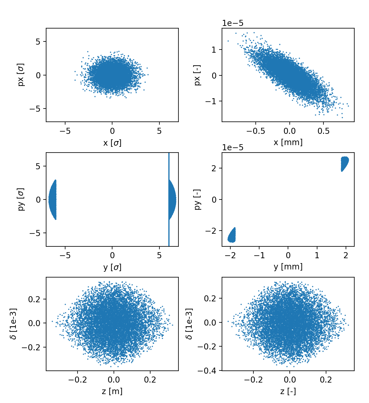
Particle distribution in normalized coordinates (left) and physical coordinates (right). See the full code generating the image.
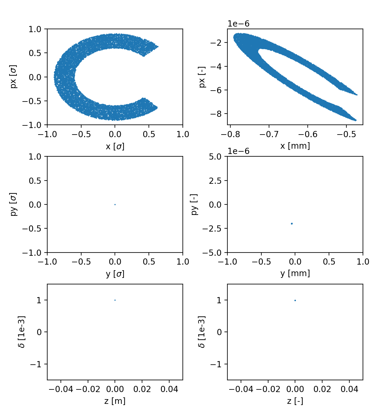
Example: Halo beam
The following example shows how to generate a distribution, which combines:
A halo distribution with an azimuthal cut in (x, px);
All particles on the closed orbit in (y, py);
All particles in the same point in (zeta, delta);
import numpy as np

import xpart as xp
import xtrack as xt

num_particles = 10000
nemitt_x = 2.5e-6
nemitt_y = 3e-6

line = xt.load('../../../xtrack/test_data/lhc_no_bb/line_and_particle.json')

line.set_particle_ref('proton', p0c=7e12)

# Horizontal plane: generate cut halo distribution
(x_in_sigmas, px_in_sigmas, r_points, theta_points
    )= xp.generate_2D_uniform_circular_sector(
                                          num_particles=num_particles,
                                          r_range=(0.6, 0.9), # sigmas
                                          theta_range=(0.25*np.pi, 1.75*np.pi))

# Vertical plane: all particles on the closed orbit
y_in_sigmas = 0.
py_in_sigmas = 0.

# Longitudinal plane: all particles off momentum by 1e-3
zeta = 0.
delta = 1e-3

# Build particles:
#    - scale with given emittances
#    - transform to physical coordinates (using 1-turn matrix)
#    - handle dispersion
#    - center around the closed orbit
particles = line.xpart.build_particles(
            zeta=zeta, delta=delta,
            x_norm=x_in_sigmas, px_norm=px_in_sigmas,
            y_norm=y_in_sigmas, py_norm=py_in_sigmas,
            nemitt_x=nemitt_x, nemitt_y=nemitt_y)

# Absolute coordinates can be inspected in particle.x, particles.px, etc.

# Tracking can be done with:
# line.track(particles, num_turns=10)

# Complete source: xpart/examples/particles_generation/002_halo.py
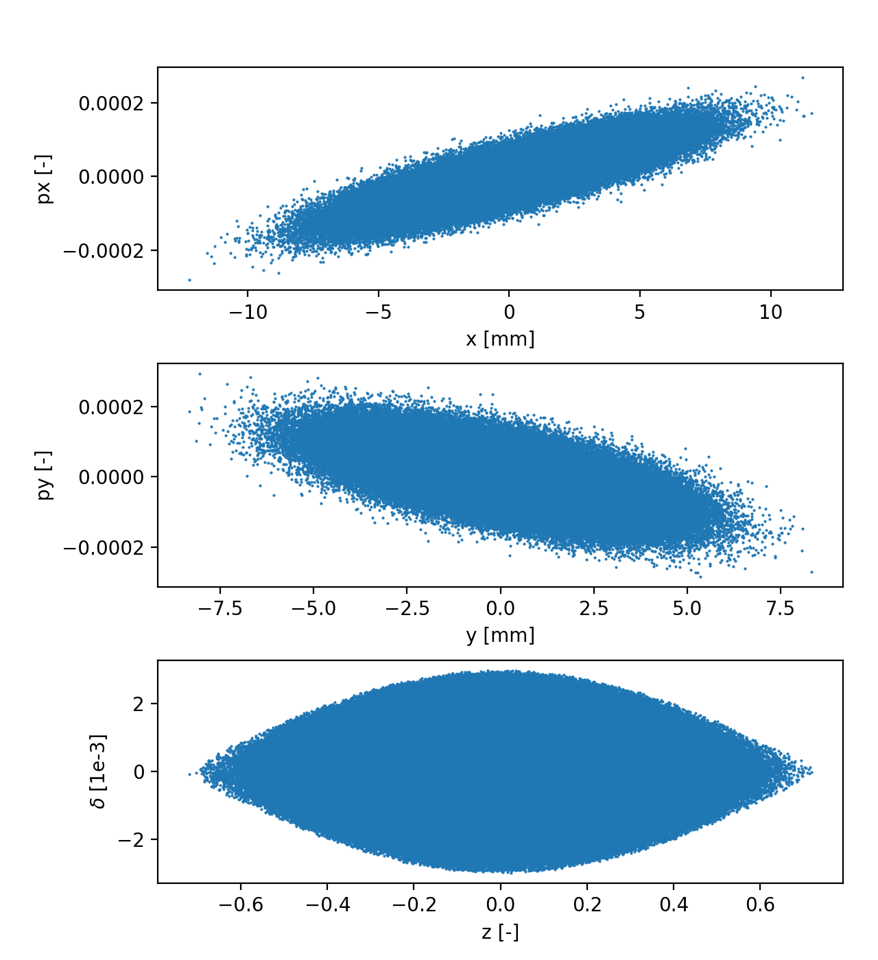
Example: Gaussian bunch
The function xpart.generate_matched_gaussian_bunch() can be used to
generate a bunch having Gaussian distribution in all coordinates and matched to
the non-linead RF bucket, as illustrated by the following example:
import numpy as np

import xtrack as xt

bunch_intensity = 1e11
sigma_z = 22.5e-2
n_part = int(5e5)
nemitt_x = 2e-6
nemitt_y = 2.5e-6

line = xt.load('../../../xtrack/test_data/sps_w_spacecharge/line_no_spacecharge_and_particle.json')
line.set_particle_ref('proton', p0c=26e9)

particles = line.xpart.generate_matched_gaussian_bunch(
         num_particles=n_part, total_intensity_particles=bunch_intensity,
         nemitt_x=nemitt_x, nemitt_y=nemitt_y, sigma_z=sigma_z)

# Complete source: xpart/examples/particles_generation/004_generate_gaussian.py
Matching distribution at custom location in the ring
The functions xtrack.Line.generate_matched_gaussian_bunch() can be used to
match a particle distribution at a custom location in the ring, as illustrated
by the following example:
import xtrack as xt

line = xt.load('../../../xtrack/test_data/lhc_no_bb/line_and_particle.json')
line.set_particle_ref('proton', p0c=7e12)

# Match distribution at a given element
particles = line.xpart.build_particles(x_norm=[0,1,2], px_norm=[0,0,0], # in sigmas
                   nemitt_x=2.5e-6, nemitt_y=2.5e-6,
                   at_element='ip2')

# Match distribution at a given s position (100m downstream of ip6)
particles = line.xpart.build_particles(x_norm=[0,1,2], px_norm=[0,0,0], # in sigmas
                   nemitt_x=2.5e-6, nemitt_y=2.5e-6,
                   at_element='ip6',
                   match_at_s=line.get_table()['s', 'ip6'] + 100
                   )

# Complete source: xpart/examples/particles_generation/006_match_at_element.py
Copying a Particles object (optionally across contexts)
The copy method allows making copies of a Particles object within the
same context or in another context. It can be used for example to transfer
Particles objects to/from GPU, as shown by the following example:
import xpart as xp
import xobjects as xo

p1 = xp.Particles(x=[1,2,3])

# Make a copy of p1 in the same context
p2 = p1.copy()

# Alter p1
p1.x += 10

# Inspect
print(p1.x) # gives [11. 12. 13.]
print(p2.x) # gives [1. 2. 3.]

# Copy across contexts
ctxgpu = xo.ContextCupy()
p3 = p1.copy(_context=ctxgpu)

# Inspect
print(p3.x[2]) # gives 13

# Complete source: xpart/examples/merge_copy_filter/001_copy.py
Saving and loading Particles objects to/from dictionary or file
The methods to_dict/from_dict and to_pandas/from_pandas allow
transforming a Particles object into a dictionary or a pandas dataframe and
back. By default the particles coordinates are transferred to CPU when using
to_dict or to_pandas.
Such methods can be used to save or load particles coordinated to/from file as shown by the following examples:
Save and load from dictionary
import numpy as np

import xobjects as xo
import xpart as xp

# Create a Particles on your selected context (default is CPU)
context = xo.ContextCupy()
part = xp.Particles(_context=context, x=[1,2,3])

# Save particles to dict
dct = part.to_dict()

# Load particles from dict
part_from_dict = xp.Particles.from_dict(dct, _context=context)

# Complete source: xpart/examples/save_and_load/000_to_from_dict.py
Save and load from json file
import numpy as np

import xobjects as xo
import xpart as xp

# Create a Particles on your selected context (default is CPU)
context = xo.ContextCupy()
part = xp.Particles(_context=context, x=[1,2,3])

# Save particles to json
import json
with open('part.json', 'w') as fid:
    json.dump(part.to_dict(), fid, cls=xo.JEncoder)

# Load particles from json file to selected context
with open('part.json', 'r') as fid:
    part_from_json= xp.Particles.from_dict(json.load(fid), _context=context)

# Complete source: xpart/examples/save_and_load/001_save_load_json.py
Save and load from pickle file
import numpy as np

import xobjects as xo
import xpart as xp

# Create a Particles on your selected context (default is CPU)
context = xo.ContextCupy()
part = xp.Particles(_context=context, x=[1,2,3])

##########
# PICKLE #
##########

# Save particles to pickle file
import pickle
with open('part.pkl', 'wb') as fid:
    pickle.dump(part.to_dict(), fid)

# Load particles from json to selected context
with open('part.pkl', 'rb') as fid:
    part_from_pkl= xp.Particles.from_dict(pickle.load(fid), _context=context)

# Complete source: xpart/examples/save_and_load/002_save_load_pickle.py
Save and load using pandas
import numpy as np

import xobjects as xo
import xpart as xp

# Create a Particles on your selected context (default is CPU)
context = xo.ContextCupy()
part = xp.Particles(_context=context, x=[1,2,3])

##############
# PANDAS/HDF #
##############

# Save particles to hdf file via pandas
import pandas as pd
df = part.to_pandas()
df.to_hdf('part.hdf', key='df', mode='w')

# Read particles from hdf file via pandas
part_from_pdhdf = xp.Particles.from_pandas(pd.read_hdf('part.hdf'))

# Complete source: xpart/examples/save_and_load/003_save_load_with_pandas.py
Merging and filtering Particles objects
Merging Particles objects
The merge method can be used to merge Particles objects as shown by the
following example:
import xpart as xp

p1 = xp.Particles(x=[1,2,3])
p2 = xp.Particles(x=[4, 5])
p3 = xp.Particles(x=6)

particles = xp.Particles.merge([p1,p2,p3])

print(particles.x) # gives [1. 2. 3. 4. 5. 6.]

# Complete source: xpart/examples/merge_copy_filter/000_merge.py
Filtering a Particles object
The filter method can be used to select a subset of particles satisfying a
logical condition defined by the user.
import xpart as xp

p1 = xp.Particles(x=[1,2,3], px=[10, 20, 30])

mask = p1.x > 1

p2 = p1.filter(mask)

print(p2.x) # gives [2. 3.]
print(p2.px) # gives [20. 30.]

# Complete source: xpart/examples/merge_copy_filter/002_filter.py
Accessing particles coordinates on GPU contexts
When working on a GPU context, the coordinate attributes of particle objects are not numpy arrays as on the CPU contexts, but specific array types associated with the specific context (e.g. cupy arrays for contexts of type ContextCupy). Although such arrays can be directly inspected to a large extent, several actions, notably plotting with matplotlib and saving to pickle or json files, are not possible without explicitly transferring the data to the CPU memory.
For this purpose we recommend to use the specific functions provided by the context in order to keep the code usable on different contexts. For example:
import xobjects as xo
import xtrack as xt

context = xo.ContextCupy()

particles = xt.Particles(_context=context, x=[1, 2, 3])

# Avoid the following (which does not work if a CPU context is chosen):
# x_cpu = particles.x.get()

# Instead use the following (which is guaranteed to work on all contexts):
x_cpu = context.nparray_from_context_array(particles.x)