Collective effects
Tracking with collective elements
A collective beam element is an element that needs access to the entire particle set (in read and/or write mode). The following example shows how to handle such elements in Xsuite.
Example
A typical example of a collective element is a space-charge interaction. We can create a space-charge beam element as follows:
import xobjects as xo
import xfields as xf

context = xo.ContextCpu()

spcharge = xf.SpaceChargeBiGaussian(_context=context,
    update_on_track = ['sigma_x', 'sigma_y'], length=2,
    longitudinal_profile=xf.LongitudinalProfileQGaussian(
        _context=context, number_of_particles=1e11, sigma_z=0.2))
This creates a space-charge element where the transverse beam sizes are updated based on the particle set at each interaction. Such an element can be included in an xtrack tracker similarly to single-particle elements.
import xtrack as xt

## Generate a simple beam line including the spacecharge element
myqf = xt.Multipole(knl=[0, 1.])
myqd = xt.Multipole(knl=[0, -1.])
mydrift = xt.Drift(length=1.)
line = xt.Line(
    elements = [myqf, mydrift, myqd, mydrift,
                spcharge,
                myqf, mydrift, myqd, mydrift,],
    element_names = ['qf1', 'drift1', 'qd1', 'drift2',
                        'spcharge'
                        'qf2', 'drift3', 'qd2', 'drift4'])

## Transfer lattice on context and compile tracking code
line.build_tracker(_context=context)

## Build particle object on context
n_part = 200
particles = xt.Particles(_context=context,
                        p0c=6500e9,
                        x=np.random.uniform(-1e-3, 1e-3, n_part),
                        px=np.random.uniform(-1e-5, 1e-5, n_part),
                        y=np.random.uniform(-2e-3, 2e-3, n_part),
                        py=np.random.uniform(-3e-5, 3e-5, n_part),
                        zeta=np.random.uniform(-1e-2, 1e-2, n_part),
                        delta=np.random.uniform(-1e-4, 1e-4, n_part),
                        )

## Track (saving turn-by-turn data)
n_turns = 100
line.track(particles, num_turns=n_turns,
            turn_by_turn_monitor=True)
How does it work?
To decide whether or not an element needs to be treated as collective, the
tracker inspects its iscollective attribute. In our example:
print(qf.iscollective)
# Gives "False"

print(spcharge.iscollective)
# Gives "True"
Based on this information, the line is divided into parts that are either collective elements or Xtrack trackers simulating groups of consecutive non-collective elements.
We can visualize this in our example:
print(line.tracker._parts)
# Gives:
# [<xtrack.tracker.Tracker object at 0x7f5ba8ce7760>,
#  <xfields.beam_elements.spacecharge.SpaceChargeBiGaussian object at 0x7f5ba8e1bd30>,
#  <xtrack.tracker.Tracker object at 0x7f5ba8ce7610>]
where the first part tracks the particles through the first portion of the machine up to the space-charge element, the second part simulates the space-charge interaction, and the third part tracks the particles from the space-charge element to the end of the line.
As all Xsuite and Xsuite-compatible beam elements need to expose a .track
method, the instruction:
line.track(particles)
is equivalent to the loop:
for pp in line.tracker._parts:
    pp.track(particles)
Any python object exposing a .track method can be used as a beam element. If the
attribute iscollective is not present, the element is handled as collective.
Xwakes: wakefields and impedances
xwakes provides wakefield and impedance elements that plug into the
Xsuite tracking environment. It offers analytic resonator wakes, wakes read from
tables, multi-bunch/multi-turn support, transverse damping, monitoring, and
MPI pipeline wiring. The list of available wakefield elements is available in
the API reference.
Quick start: resonator wake on a single bunch
import numpy as np
import xtrack as xt
import xwakes as xw

# Build a wake as the sum of dipolar and quadrupolar resonators
wf_dip_1 = xw.WakeResonator(kind='dipolar_x', r=1e8, q=1e5, f_r=1e3)
wf_dip_2 = xw.WakeResonator(kind='dipolar_x', r=5e7, q=5e4, f_r=5e2)
wf_quad_1 = xw.WakeResonator(kind='quadrupolar_x', r=2e7, q=8e4, f_r=2e3)
wf_quad_2 = xw.WakeResonator(kind='quadrupolar_y', r=3e7, q=6e4, f_r=1.5e3)
wf = wf_dip_1 + wf_dip_2 + wf_quad_1 + wf_quad_2

# Configure for tracking: zeta range and number of slices
wf.configure_for_tracking(
    zeta_range=(-0.1, 0.1),  # meters
    num_slices=100
)

# Simple accelerator lattice: one turn map plus wake
one_turn = xt.LineSegmentMap(length=26000, betx=50., bety=40., qx=62.28, qy=62.31,
                             longitudinal_mode='linear_fixed_qs', qs=1e-3, bets=100)
line = xt.Line(elements=[one_turn, wf], element_names=['one_turn', 'wake'])
line.set_particle_ref('proton', p0c=7e12)

# One particle per slice, give it an offset, track once and inspect the kick
particles = line.build_particles(
    x=0, px=0, y=0, py=0,
    zeta=wf.slicer.zeta_centers.flatten(),
)
particles.x += 1e-3  # mm-level offset

# Track one turn
line.track(particles, num_turns=1)
configure_for_tracking prepares the internal slicer and wake tracker
(zeta_range, num_slices) and must be called before tracking. Summing
wakes works naturally: wf_total = wf1 + wf2 + wf3; the combined wake is
configured once and used like a single element.
Wakefield definitions
Transverse wakefields are defined such that the transverse kicks are given by:
where \(\bar{x}(z)\) and \(\bar{y}(z)\) are the transverse centroids, and \(\lambda(z)\) is the line density. The exponents \((i,j)\) belong to the source moments, while \((k,l)\) apply to the test particle offsets.
Longitudinal kicks are defined so that the change in momentum deviation is:
with the sign convention that a positive wake causes energy loss.
Each predefined kind maps to a plane and to a set of source exponents
\((i,j)\) and test exponents \((k,l)\), following \(W^{i,j,k,l}\) in
the formulas above. The available kinds are listed below:
kind |
plane |
source_exponents |
test_exponents |
meaning |
|---|---|---|---|---|
|
z |
(0, 0) |
(0, 0) |
longitudinal |
|
x |
(0, 0) |
(0, 0) |
constant x |
|
y |
(0, 0) |
(0, 0) |
constant y |
|
x |
(1, 0) |
(0, 0) |
dipolar / driving x |
|
y |
(0, 1) |
(0, 0) |
dipolar / driving y |
|
x |
(0, 1) |
(0, 0) |
dipolar / driving xy |
|
y |
(1, 0) |
(0, 0) |
dipolar / driving yx |
|
x |
(0, 0) |
(1, 0) |
quadrupolar / detuning x |
|
y |
(0, 0) |
(0, 1) |
quadrupolar / detuning y |
|
x |
(0, 0) |
(0, 1) |
quadrupolar / detuning xy |
|
y |
(0, 0) |
(1, 0) |
quadrupolar / detuning yx |
Wakefield objects can be initialized in different ways, as illustrated by the following examples.
- Single component
# Horizontal dipolar resonator
w1 = xw.WakeResonator(kind='dipolar_x', r=1e8, q=1e5, f_r=1e9)
- Multiple components (list/tuple)
# Horizontal + vertical dipolar with same r/q/f_r
w2 = xw.WakeResonator(kind=['dipolar_x', 'dipolar_y'],
                      r=1e8, q=1e5, f_r=1e9)
- Weighted components (dict)
# Scale horizontal twice as strong as vertical
w3 = xw.WakeResonator(kind={'dipolar_x': 2.0, 'dipolar_y': 1.0},
                      r=1e8, q=1e5, f_r=1e9)
- Using Yokoya factors
# Flat chamber (horizontal) yokoya factors expanded into the right components
w4 = xw.WakeResonator(kind=xw.Yokoya('flat_horizontal'),
                      r=1e8, q=1e5, f_r=1e9)
- Custom polynomial term
# Custom plane/exponents without a predefined kind entry
w5 = xw.WakeResonator(
    plane='y',
    source_exponents=(1, 0),  # x_source^1 y_source^0
    test_exponents=(0, 2),    # x_test^0 y_test^2
    r=1e8, q=1e5, f_r=1e9)
- Combine and configure
w = w1 + w2 + w3.components[0]  # mix whole wakes and single components
w.configure_for_tracking(zeta_range=(-0.1, 0.1), num_slices=200)
Building wakes from tables
The class WakeFromTable builds wakefields from tabulated data in the time domain.
Columns must correspond to the wakefield kinds defined above. The function
xw.read_headtail_file can be used to read HEADTAIL-format files, as illustrated
in the following examples.
import pathlib
import xwakes as xw

test_data = pathlib.Path(__file__).parent / 'test_data' / 'HLLHC_wake.dat'
columns = ['time', 'longitudinal', 'dipolar_x', 'dipolar_y',
           'quadrupolar_x', 'quadrupolar_y']

table = xw.read_headtail_file(test_data, columns)

# use only dipolar terms
wf = xw.WakeFromTable(table, columns=['dipolar_x', 'dipolar_y'])

# Configure for tracking
wf.configure_for_tracking(zeta_range=(-0.4, 0.4), num_slices=100)

# Track as usual in a line
# ...
Defining custom wakes
For forms not covered by the built-in components, you can build a Component directly
from a wake callable in the time domain. Provide the plane of the kick, and the polynomial
exponents applied to the source/test offsets (source_exponents for the source particle,
test_exponents for the particle being kicked). The wake callable receives time t in
seconds; enforce causality by zeroing t <= 0. Wrap one or more components in xw.Wake
and configure it like any other wake.
import numpy as np
import xwakes as xw

a, b, c = 1.0e9, 0.1e9, 2.0  # frequency, damping rate, amplitude

def wake_vs_t(t):
    t = np.atleast_1d(t)
    out = c * np.sin(a * t) * np.exp(-b * t)
    out[t <= 0] = 0.0  # causal wake
    return out

custom_component = xw.Component(
    wake=wake_vs_t,
    plane='y',
    source_exponents=(2, 0),
    test_exponents=(1, 1),
    name="Example damped sine wake",
)

custom_wake = xw.Wake(components=[custom_component])

# Inspect the zeta-domain wake or combine with other components
zeta = np.linspace(-10, 10, 500)
values = custom_component.function_vs_zeta(zeta, beta0=0.7)
custom_wake.configure_for_tracking(zeta_range=(-0.1, 0.1), num_slices=200)
The snippet mirrors xwakes/examples/003_custom_wake.py; you can mix these components with
resonators or tables via custom_wake + other_wake.
Multi-bunch, multi-turn wakes
configure_for_tracking accepts multi-bunch/multi-turn options:
filling_scheme: array of 0/1 slots (length = number of RF buckets considered)bunch_spacing_zeta: spacing between buckets in metersnum_turnsandcircumference: enable multi-turn wake memory
Example (two bunches, one-turn memory):
import numpy as np
import xwakes as xw
import xpart as xp
import xtrack as xt

filling_scheme = np.zeros(3564, dtype=int)
filling_scheme[0] = filling_scheme[1] = 1

wf = xw.WakeResonator(kind='dipolar_x', r=1e8, q=1e5, f_r=600e6)
wf.configure_for_tracking(
    zeta_range=(-0.2, 0.2),
    num_slices=200,
    filling_scheme=filling_scheme,
    bunch_spacing_zeta=26658.8832 / 3564,
    num_turns=1,
    circumference=26658.8832,
)

# Simple one-turn map and line
one_turn = xt.LineSegmentMap(
    length=26658.8832, betx=70., bety=80., qx=62.31, qy=60.32,
    longitudinal_mode='nonlinear', qs=2e-3, bets=731.27)
line = xt.Line([one_turn, wf], element_names=['one_turn', 'wake'])
line.particle_ref = xt.Particles(p0c=7e12)

# Generate a matched two-bunch beam and track
particles = xp.generate_matched_gaussian_multibunch_beam(
    line=line, filling_scheme=filling_scheme,
    bunch_num_particles=100_000, bunch_intensity_particles=2.3e11,
    nemitt_x=2e-6, nemitt_y=2e-6, sigma_z=0.08,
    bucket_length=26658.8832 / 35640, bunch_spacing_buckets=10,
)
line.track(particles, num_turns=10)
Space charge
Xsuite can be used to perform simulations including space-charge effects. Three modes can be used to simulate the space-charge forces:
Frozen: A fixed Gaussian bunch distribution is used to compute the space-charge forces.
Quasi-frozen: Forces are computed assuming a Gaussian distribution. The properties of the distribution (transverse r.m.s. sizes, transverse positions) are updated at each interaction based on the particle distribution.
PIC: The Particle In Cell method is used to compute the forces acting among particles. No assumption is made on the bunch shape.
The last two options constitute collective interactions. As discussed in the dedicated section, the Xtrack Line works such that particles are tracked asynchronously by separate threads in the non-collective sections of the sequence and are regrouped at each collective element (in PIC or quasi-frozen space-charge lenses).
The following example illustrates how to configure and run a space-charge simulation.
The variable mode is used to switch between frozen, quasi-frozen and PIC.
See also: xfields.install_spacecharge_frozen(),
xfields.replace_spacecharge_with_quasi_frozen(),
xfields.replace_spacecharge_with_PIC().
Example
import json
import numpy as np

import xobjects as xo
import xpart as xp
import xtrack as xt
import xfields as xf

############
# Settings #
############

fname_line = ('../../test_data/sps_w_spacecharge/'
                  'line_no_spacecharge_and_particle.json')

bunch_intensity = 1e11/3 # Need short bunch to avoid bucket non-linearity
                         # to compare frozen/quasi-frozen and PIC
sigma_z = 22.5e-2/3
nemitt_x=2.5e-6
nemitt_y=2.5e-6
n_part=int(1e6)
num_turns=32

num_spacecharge_interactions = 540

# Available modes: frozen/quasi-frozen/pic
# mode = 'pic'
mode = 'quasi-frozen'

# Choose solver between `FFTSolver2p5DAveraged` and `FFTSolver2p5D`
pic_solver = 'FFTSolver2p5DAveraged'

####################
# Choose a context #
####################

context = xo.ContextCpu()
#context = xo.ContextCupy()
#context = xo.ContextPyopencl('0.0')

print(context)

#############
# Load line #
#############

with open(fname_line, 'r') as fid:
     input_data = json.load(fid)
line = xt.Line.from_dict(input_data['line'])
line.particle_ref = xt.Particles.from_dict(input_data['particle'])


line.build_tracker(_context=context, compile=False)

#############################################
# Install spacecharge interactions (frozen) #
#############################################

lprofile = xf.LongitudinalProfileQGaussian(
        number_of_particles=bunch_intensity,
        sigma_z=sigma_z,
        z0=0.,
        q_parameter=1.)

line.xfields.spacecharge_install_frozen(
                   longitudinal_profile=lprofile,
                   nemitt_x=nemitt_x, nemitt_y=nemitt_y,
                   sigma_z=sigma_z,
                   num_spacecharge_interactions=num_spacecharge_interactions,
                   )

#################################
# Switch to PIC or quasi-frozen #
#################################

if mode == 'frozen':
    pass # Already configured in line
elif mode == 'quasi-frozen':
    line.xfields.spacecharge_replace_with_quasi_frozen(
                                    update_mean_x_on_track=True,
                                    update_mean_y_on_track=True)
elif mode == 'pic':
    pic_collection, all_pics = line.xfields.spacecharge_replace_with_pic(
        n_sigmas_range_pic_x=8,
        n_sigmas_range_pic_y=8,
        nx_grid=256, ny_grid=256, nz_grid=100,
        n_lims_x=7, n_lims_y=3,
        z_range=(-3*sigma_z, 3*sigma_z),
        solver=pic_solver)
else:
    raise ValueError(f'Invalid mode: {mode}')

#################
# Build Tracker #
#################

line.build_tracker(_context=context)

######################
# Generate particles #
######################

# Build a line without spacecharge (recycling the track kernel)
line_sc_off = line.filter_elements(exclude_types_starting_with='SpaceCh')
line_sc_off.build_tracker(track_kernel=line.tracker.track_kernel)

# (we choose to match the distribution without accounting for spacecharge)
particles = xp.generate_matched_gaussian_bunch(line=line_sc_off,
         num_particles=n_part, total_intensity_particles=bunch_intensity,
         nemitt_x=nemitt_x, nemitt_y=nemitt_y, sigma_z=sigma_z)

####################################################
# Check that everything is on the selected context #
####################################################

assert particles._context == context
assert len(set([ee._buffer for ee in line.elements])) == 1 # All on same context
assert line._context == context

#########
# Track #
#########
line.track(particles, num_turns=num_turns, with_progress=1)

# Complete source: xtrack/examples/spacecharge/000_spacecharge_example.py
Beam-beam
Weak-strong 2D
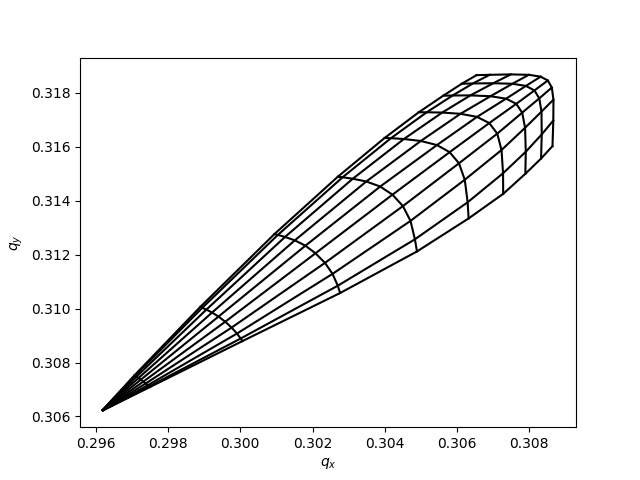
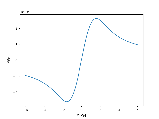
The example below shows how to introduce a 2D beam-beam element in a line and perform a few studies based on tracking. The 2D beam-beam element provides a kick based on the Bassetti-Erskine formula neglecting any longitudinal variations of the beam-beam force.
import numpy as np
from matplotlib import pyplot as plt
import xobjects as xo
import xtrack as xt
import xfields as xf
import xpart as xp

context = xo.ContextCpu(omp_num_threads=0)

# Machine and beam parameters
n_macroparticles = int(1e4)
bunch_intensity = 2.3e11
nemitt_x = 2E-6
nemitt_y = 2E-6
p0c = 7e12
gamma = p0c/xp.PROTON_MASS_EV
physemit_x = nemitt_x/gamma
physemit_y = nemitt_y/gamma
beta_x = 1.0
beta_y = 1.0
sigma_z = 0.08
sigma_delta = 1E-4
beta_s = sigma_z/sigma_delta
Qx = 0.31
Qy = 0.32
Qs = 2.1E-3

##############################
# Plot the beam-beam force   #
##############################

# Particles algined on the x axis
particles = xp.Particles(_context=context,
    p0c=p0c,
    x=np.sqrt(physemit_x*beta_x)*np.linspace(-6,6,n_macroparticles),
    px=np.zeros(n_macroparticles),
    y=np.zeros(n_macroparticles),
    py=np.zeros(n_macroparticles),
    zeta=np.zeros(n_macroparticles),
    delta=np.zeros(n_macroparticles),
)
# Definition of the beam-beam force based on the other beam's
# properties (here assumed identical to the tracked beam)
# Note that the arguments 'Sigma' are sigma**2
bbeam = xf.BeamBeamBiGaussian2D(
            _context=context,
            other_beam_q0 = particles.q0,
            other_beam_beta0 = particles.beta0[0],
            other_beam_num_particles = bunch_intensity,
            other_beam_Sigma_11 = physemit_x*beta_x,
            other_beam_Sigma_33 = physemit_y*beta_y)

# Build line and tracker with only the beam-beam element
elements = [bbeam]
line = xt.Line(elements=elements)
line.particle_ref = xp.Particles(mass0=xp.PROTON_MASS_EV, p0c=7e12)
line.build_tracker()
# track on turn
line.track(particles,num_turns=1)
#plot the resulting change of px
plt.figure()
plt.plot(particles.x/np.sqrt(physemit_x*beta_x),particles.px)
plt.xlabel(r'x [$\sigma_x$]')
plt.ylabel(r'$\Delta p_x$')

##############################
# Tune footprint             #
##############################

# Build linear lattice
arc = xt.LineSegmentMap(
        betx = beta_x,bety = beta_y,
        qx = Qx, qy = Qy,bets = beta_s, qs=Qs)
# Build line and tracker with a beam-beam element and linear lattice
elements = [bbeam,arc]
line = xt.Line(elements=elements)
line.particle_ref = xp.Particles(mass0=xp.PROTON_MASS_EV, p0c=7e12)
line.build_tracker()
# plot footprint
plt.figure()
fp0 = line.get_footprint(nemitt_x=nemitt_x, nemitt_y=nemitt_y)
fp0.plot(color='k')

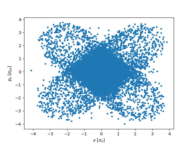
##############################
# Phase space distorion      #
##############################

# Initialise particles randomly in 6D phase space
particles = xp.Particles(_context=context,
    p0c=p0c,
    x=np.sqrt(physemit_x*beta_x)*(np.random.randn(n_macroparticles)),
    px=np.sqrt(physemit_x/beta_x)*np.random.randn(n_macroparticles),
    y=np.sqrt(physemit_y*beta_y)*(np.random.randn(n_macroparticles)),
    py=np.sqrt(physemit_y/beta_y)*np.random.randn(n_macroparticles),
    zeta=sigma_z*np.random.randn(n_macroparticles),
    delta=sigma_delta*np.random.randn(n_macroparticles),
)

# Change the tune to better visualise the 4th order resonance
arc.qx=0.255
# Track
line.track(particles,num_turns=10000)
# Plot phase space
plt.figure()
plt.plot(particles.x/np.sqrt(physemit_x*beta_x),particles.px/np.sqrt(physemit_x/beta_x),'.')
plt.xlabel('$x$ [$\sigma_x$]')
plt.ylabel('$p_x$ [$\sigma_{px}$]')
plt.show()

# Complete source: xfields/examples/002_beambeam/010_beambeam2d_weakstrong.py
Weak-strong 3D
The 3D beam-beam element can be used similarly, replacing the instantiation of the beam-beam element as in the example below. This element takes into account longitudinal variations of the beam-beam force (hourglass, crossing angle) based on a longitudinal slicing of the beam (Hirata’s method) handled by the xfields.beam_elements.TempSlicer.
# Number of longitudinal slices
n_slices = 21
# Slicer used to determine the position and charge of the slices
# based on an optimised algorithm by D. Shatilov. (other options are also possible)
slicer = xf.TempSlicer(n_slices=n_slices, sigma_z=sigma_z, mode="shatilov")
bbeam = xf.BeamBeamBiGaussian3D(
            _context=context,
            other_beam_q0 = particles.q0,
            # Full crossing angle at the IP in rad
            phi = 500.0E-2,
            # Roll angle of the crossing angle in rad (0 -> horizontal, pi/2 -> vertical)
            alpha = 0.0,
            # charge in each slice
            slices_other_beam_num_particles = slicer.bin_weights * bunch_intensity,
            # longitudinal position of the slice
            slices_other_beam_zeta_center = slicer.bin_centers,
            # transverse sizes of the slices at the IP (squarred)
            slices_other_beam_Sigma_11 = np.zeros(n_slices,dtype=float)+physemit_x*beta_x,
            slices_other_beam_Sigma_12 = np.zeros(n_slices,dtype=float),
            slices_other_beam_Sigma_13 = np.zeros(n_slices,dtype=float),
            slices_other_beam_Sigma_14 = np.zeros(n_slices,dtype=float),
            slices_other_beam_Sigma_22 = np.zeros(n_slices,dtype=float)+physemit_x/beta_x,
            slices_other_beam_Sigma_23 = np.zeros(n_slices,dtype=float),
            slices_other_beam_Sigma_24 = np.zeros(n_slices,dtype=float),
            slices_other_beam_Sigma_33 = np.zeros(n_slices,dtype=float)+physemit_y*beta_y,
            slices_other_beam_Sigma_34 = np.zeros(n_slices,dtype=float),
            slices_other_beam_Sigma_44 = np.zeros(n_slices,dtype=float)+physemit_y/beta_y)
Strong-strong (soft-Gaussian)
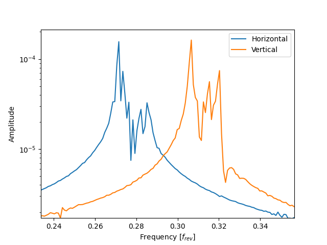
Strong-strong simulations can be performed using the Pipeline for multibunch simulations, as in the example below.
import time

import numpy as np
from matplotlib import pyplot as plt
from mpi4py import MPI
import xobjects as xo
import xtrack as xt
import xfields as xf
import xpart as xp

context = xo.ContextCpu(omp_num_threads=0)

####################
# Pipeline manager #
####################

# Retrieving MPI info
comm = MPI.COMM_WORLD
nprocs = comm.Get_size()
my_rank   = comm.Get_rank()

# Building the pipeline manager based on a MPI communicator
pipeline_manager = xt.PipelineManager(comm)
if nprocs >= 2:
    # Add information about the Particles instance that require
    # communication through the pipeline manager.
    # Each Particles instance must be identifiable by a unique name
    # The second argument is the MPI rank in which the Particles object
    # lives.
    pipeline_manager.add_particles('B1b1',0)
    pipeline_manager.add_particles('B2b1',1)
    # Add information about the elements that require communication
    # through the pipeline manager.
    # Each Element instance must be identifiable by a unique name
    # All Elements are instanciated in all ranks
    pipeline_manager.add_element('IP1')
    pipeline_manager.add_element('IP2')
else:
    print('Need at least 2 MPI processes for this test')
    exit()

#################################
# Generate particles            #
#################################

n_macroparticles = int(1e4)
bunch_intensity = 2.3e11
physemit_x = 2E-6*0.938/7E3
physemit_y = 2E-6*0.938/7E3
beta_x_IP1 = 1.0
beta_y_IP1 = 1.0
beta_x_IP2 = 1.0
beta_y_IP2 = 1.0
sigma_z = 0.08
sigma_delta = 1E-4
beta_s = sigma_z/sigma_delta
Qx = 0.285
Qy = 0.32
Qs = 2.1E-3

#Offsets [sigma] the two beams with opposite direction
#to enhance oscillation of the pi-mode
mean_x_init = 0.1
mean_y_init = 0.1

p0c = 7000e9

print('Initialising particles')
if my_rank == 0:
    particles = xp.Particles(_context=context,
        p0c=p0c,
        x=np.sqrt(physemit_x*beta_x_IP1)
            *(np.random.randn(n_macroparticles)+mean_x_init),
        px=np.sqrt(physemit_x/beta_x_IP1)
            *np.random.randn(n_macroparticles),
        y=np.sqrt(physemit_y*beta_y_IP1)
            *(np.random.randn(n_macroparticles)+mean_y_init),
        py=np.sqrt(physemit_y/beta_y_IP1)
            *np.random.randn(n_macroparticles),
        zeta=sigma_z*np.random.randn(n_macroparticles),
        delta=sigma_delta*np.random.randn(n_macroparticles),
        weight=bunch_intensity/n_macroparticles
    )
    # Initialise the Particles object with its unique name
    # (must match the info provided to the pipeline manager)
    particles.init_pipeline('B1b1')
    # Keep in memory the name of the Particles object with which this
    # rank will communicate
    # (must match the info provided to the pipeline manager)
    partner_particles_name = 'B2b1'
elif my_rank == 1:
    particles = xp.Particles(_context=context,
        p0c=p0c,
        x=np.sqrt(physemit_x*beta_x_IP1)
            *(np.random.randn(n_macroparticles)+mean_x_init),
        px=np.sqrt(physemit_x/beta_x_IP1)
            *np.random.randn(n_macroparticles),
        y=np.sqrt(physemit_y*beta_y_IP1)
            *(np.random.randn(n_macroparticles)-mean_y_init),
        py=np.sqrt(physemit_y/beta_y_IP1)
            *np.random.randn(n_macroparticles),
        zeta=sigma_z*np.random.randn(n_macroparticles),
        delta=sigma_delta*np.random.randn(n_macroparticles),
        weight=bunch_intensity/n_macroparticles
    )
    # Initialise the Particles object with its unique name
    # (must match the info provided to the pipeline manager)
    particles.init_pipeline('B2b1')
    # Keep in memory the name of the Particles object with which this
    # rank will communicate
    # (must match the info provided to the pipeline manager)
    partner_particles_name = 'B1b1'
else:
    # Stop the execution of ranks that are not needed
    print('No need for rank',my_rank)
    exit()

#############
# Beam-beam #
#############

nb_slice = 11
slicer = xf.TempSlicer(sigma_z=sigma_z, n_slices=nb_slice)
config_for_update_IP1=xf.ConfigForUpdateBeamBeamBiGaussian3D(
   pipeline_manager=pipeline_manager,
   element_name='IP1', # The element name must be unique and match the
                       # one given to the pipeline manager
   partner_particles_name = partner_particles_name, # the name of the
                       # Particles object with which to collide
   slicer=slicer,
   update_every=1 # Setup for strong-strong simulation
   )
config_for_update_IP2=xf.ConfigForUpdateBeamBeamBiGaussian3D(
   pipeline_manager=pipeline_manager,
   element_name='IP2', # The element name must be unique and match the
                       #  one given to the pipeline manager
   partner_particles_name = partner_particles_name, # the name of the
                       #Particles object with which to collide
   slicer=slicer,
   update_every=1 # Setup for strong-strong simulation
   )


print('build bb elements...')
bbeamIP1 = xf.BeamBeamBiGaussian3D(
            _context=context,
            other_beam_q0 = particles.q0,
            phi = 500E-6,alpha=0.0,
            config_for_update = config_for_update_IP1)

bbeamIP2 = xf.BeamBeamBiGaussian3D(
            _context=context,
            other_beam_q0 = particles.q0,
            phi = 500E-6,alpha=np.pi/2,
            config_for_update = config_for_update_IP2)

#################################################################
# arcs (here they are all the same with half the phase advance) #
#################################################################

arc12 = xt.LineSegmentMap(
        betx = beta_x_IP1,bety = beta_y_IP1,
        qx = Qx/2, qy = Qy/2,bets = beta_s, qs=Qs/2)

arc21 = xt.LineSegmentMap(
        betx = beta_x_IP1,bety = beta_y_IP1,
        qx = Qx/2, qy = Qy/2,bets = beta_s, qs=Qs/2)

#################################################################
# Tracker                                                       #
#################################################################

# In this example there is one Particles object per rank
# We build its line and tracker as usual
elements = [bbeamIP1,arc12,bbeamIP2,arc21]
line = xt.Line(elements=elements)
line.build_tracker()
# A pipeline branch is a line and Particles object that will
# be tracked through it
branch = xt.PipelineBranch(line, particles)
# The multitracker can deal with a set of branches (here only one)
multitracker = xt.PipelineMultiTracker(branches=[branch])

#################################################################
# Tracking  (Same as usual)                                     #
#################################################################
print('Tracking...')
time0 = time.time()
nTurn = 1024
multitracker.track(num_turns=nTurn,turn_by_turn_monitor=True)
print('Done with tracking.',(time.time()-time0)/1024,'[s/turn]')


#################################################################
# Post-processing: raw data and spectrum                        #
#################################################################

# Show beam oscillation spectrum (only one rank)
if my_rank == 0:
    positions_x_b1 = np.average(line.record_last_track.x,axis=0)
    positions_y_b1 = np.average(line.record_last_track.y,axis=0)
    plt.figure(1)
    freqs = np.fft.fftshift(np.fft.fftfreq(nTurn))
    mask = freqs > 0
    myFFT = np.fft.fftshift(np.fft.fft(positions_x_b1))
    plt.semilogy(freqs[mask], (np.abs(myFFT[mask])),label='Horizontal')
    myFFT = np.fft.fftshift(np.fft.fft(positions_y_b1))
    plt.semilogy(freqs[mask], (np.abs(myFFT[mask])),label='Vertical')
    plt.xlabel('Frequency [$f_{rev}$]')
    plt.ylabel('Amplitude')
    plt.legend(loc=0)
    plt.show()

# Complete source: xfields/examples/002_beambeam/006_beambeam6d_strongstrong_pipeline_MPI2Procs.py
In collisions featuring a low disruption (i.e. the beam moments do not vary significantly during the interaction), the quasi-strong-strong (aka frozen-strong-strong) model may be enabled by setting the argument ‘quasistrongstrong
= True’ in xfields.beam_elements.ConfigForUpdate*. In this configuration, the beam moments are computed once at the start of the collision and kept constant throughout the collision, thus reducing the computing load. The argument ‘update_every’ makes it possible to further reduce the computing load by keeping the moments for the given number of turns. This model is suitable for effects that build up over many turns. (more details in https://accelconf.web.cern.ch/eefact2022/papers/wezat0102.pdf)
For 2D beam-beam interactions, the beam-beam element and the xfields.beam_elements.ConfigForUpdate* have to be redefined as in the example below.
config_for_update_b1_IP1=xf.ConfigForUpdateBeamBeamBiGaussian2D(
   pipeline_manager=pipeline_manager,
   element_name='IP1',
   partner_particles_name = 'B2b1',
   update_every=1
   )
config_for_update_b2_IP1=xf.ConfigForUpdateBeamBeamBiGaussian2D(
   pipeline_manager=pipeline_manager,
   element_name='IP1',
   partner_particles_name = 'B1b1',
   update_every=1
   )
bbeamIP1_b1 = xf.BeamBeamBiGaussian2D(
            _context=context,
            other_beam_q0 = particles_b2.q0,
            other_beam_beta0 = particles_b2.beta0[0],
            config_for_update = config_for_update_b1_IP1)
bbeamIP1_b2 = xf.BeamBeamBiGaussian2D(
            _context=context,
            other_beam_q0 = particles_b1.q0,
            other_beam_beta0 = particles_b1.beta0[0],
            config_for_update = config_for_update_b2_IP1)
Poisson Solver
Particle-in-cell simulations using a Poisson solver for the beam-beam interaction are currently not implemented in Xfields.
Beam-beam in a real lattice
Similarly to the examples above, beam-beam elements can be introduced into the lattice of a full machine. Several tools exist to ease the setup of beam-beam interactions in a collider lattice: Xmask. An example snippet is shown below where an Xtrack lattice in JSON format is loaded and a weak-strong beam-beam element is inserted at the marker “ip.1”.
path     = "/path/to/lattice"
seq_name = "lattice.json"
seq_path = os.path.join(path, seq_name)

 with open(seq_path, 'r') as f:
     line = xt.Line.from_dict(json.load(f))

# define slicer
slicer = xf.TempSlicer(n_slices=n_slices, sigma_z=sigma_z, mode=binning_mode)

# define weakstrong beambeam element (n*[x] yields a list with n elements each of which is x, e.g. 3*[5]=[5,5,5])
el_beambeam = xf.BeamBeamBiGaussian3D(
         _context=context,
         config_for_update = None,
         other_beam_q0=other_beam_q0,
         phi=phi, # half-crossing angle in radians
         alpha=alpha, # crossing plane in radians
         # slice intensity [num. real particles] number of slices inferred from the length of this list
         slices_other_beam_num_particles = slicer.bin_weights * nb,
         # unboosted opposing (strong) beam moments
         slices_other_beam_zeta_center = slicer.bin_centers,
         slices_other_beam_Sigma_11    = n_slices*[ sigma_x**2], # Beam sizes for the other beam, assuming the same value for all slices
         slices_other_beam_Sigma_22    = n_slices*[sigma_px**2],
         slices_other_beam_Sigma_33    = n_slices*[ sigma_y**2],
         slices_other_beam_Sigma_44    = n_slices*[sigma_py**2],
         # only if beamstrahlung on
         slices_other_beam_zeta_bin_width_star_beamstrahlung = None if not beamstrahlung_on else slicer.bin_widths_beamstrahlung / np.cos(phi),  # boosted dz
         # has to be set (0 in most cases) if config_for_update = None
         slices_other_beam_Sigma_12     = n_slices*[0],
         slices_other_beam_Sigma_34     = n_slices*[0],
         slices_other_beam_pzeta_center = n_slices*[pzeta], # important when tapering (FCC-ee specific)
     )

element_name = "ip.1"  # this is the marker name of an IP in the lattice where the beam-beam element will be inserted
element_line_index = line.element_names.index(element_name)  # get the array index of the element "ip.1"
line.insert_element(index=element_line_index, element=el_beambeam, name='beambeam')
Intra-Beam Scattering
Analytical Growth Rates
The following example illustrates how to obtain Intra-Beam Scattering growth rates in Xsuite.
The functionality is exposed directly through xtrack.TwissTable and can make use of two different formalisms: Nagaitsev and Bjorken-Mtingwa.
The former provides a computationally efficient approach but does not account for vertical dispersion, while the latter correctly accounts for it but is slower.
See also: xtrack.twiss.TwissTable.get_ibs_growth_rates()
import xtrack as xt

##########################
# Load xt.Line from file #
##########################

line = xt.load( "../../../xtrack/test_data/lhc_no_bb/line_and_particle.json")
line.set_particle_ref('proton', p0c=7e12)
tw = line.twiss(method="4d")

#####################
# Define parameters #
#####################

# Line is for LHC protons at top energy
bunch_intensity: int = int(1.8e11)
nemitt_x: float = 1.8e-6
nemitt_y: float = 1.8e-6
sigma_delta: float = 4.71e-5
bunch_length: float = 3.75e-2

###################################
# Get growth rates with Nagaitsev #
###################################

nag_growth_rates = tw.get_ibs_growth_rates(
    formalism="nagaitsev",
    total_beam_intensity=bunch_intensity,
    nemitt_x=nemitt_x,
    nemitt_y=nemitt_y,
    sigma_delta=sigma_delta,
    bunch_length=bunch_length,
    bunched=True,
)

#########################################
# Get growth rates with Bjorken-Mtingwa #
#########################################

bm_growth_rates = tw.get_ibs_growth_rates(
    formalism="bjorken-mtingwa",  # also accepts "b&m"
    total_beam_intensity=bunch_intensity,
    nemitt_x=nemitt_x,
    nemitt_y=nemitt_y,
    sigma_delta=sigma_delta,
    bunch_length=bunch_length,
    bunched=True,
)

##########################################################
# Compare: we expect Nagaitsev to be wrong in horizontal #
##########################################################

print()
print("Computed from normalized emittances:")
print("------------------------------------")
print(f"Nagaitsev:       {nag_growth_rates}")
print(f"Bjorken-Mtingwa: {bm_growth_rates}")

# Computed from normalized emittances:
# ------------------------------------
# Nagaitsev:       IBSAmplitudeGrowthRates(Kx=3.12e-05, Ky=-1.14e-09, Kz=0.000155)
# Bjorken-Mtingwa: IBSAmplitudeGrowthRates(Kx=3.11e-05, Ky=5.52e-07, Kz=0.000155)

# Complete source: xfields/examples/005_ibs/001_growth_rates_with_vdisp.py
Amplitude and Emittance Conventions
For consistency with the computed Synchrotron Radiation damping times, in Xsuite the IBS amplitude growth rates are computed. The following short example shows how to switch between the amplitude and emittance growth rates should one need to.
import xtrack as xt

##########################
# Load xt.Line from file #
##########################

line = xt.load("../../../xtrack/test_data/sps_ions/line_and_particle.json")
tw = line.twiss(method="4d")

#####################
# Define parameters #
#####################

# Line is for SPS ions at injection
bunch_intensity: int = int(3.5e8)
nemitt_x: float = 1.2612e-6
nemitt_y: float = 0.9081e-6
sigma_delta: float = 3.59e-4
bunch_length: float = 19.51e-2

####################
# Get growth rates #
####################

# There is no vertical dispersion so Nagaitsev
# will be correct in vertical
amp_growth_rates = tw.get_ibs_growth_rates(
    formalism="nagaitsev",
    total_beam_intensity=bunch_intensity,
    nemitt_x=nemitt_x,
    nemitt_y=nemitt_y,
    sigma_delta=sigma_delta,
    bunch_length=bunch_length,
    bunched=True,
)

##########################################################
# Converting between amplitude and emittance conventions #
##########################################################

# Notice how, when printing the returned object, it states
# the growth rates are given in amplitude convention
print(amp_growth_rates)
# IBSAmplitudeGrowthRates(Kx=0.000518, Ky=0.00552, Kz=0.00402)

# Methods are implemented to convert to the emittance convention
emit_growth_rates = amp_growth_rates.to_emittance_growth_rates()
print(emit_growth_rates)
# IBSEmittanceGrowthRates(Kx=0.00104, Ky=0.011, Kz=0.00803)

# It is also possible to convert back to the amplitude convention
print(f"Initial:         {amp_growth_rates}")
print(f"Converted twice: {emit_growth_rates.to_amplitude_growth_rates()}")
# Initial:         IBSAmplitudeGrowthRates(Kx=0.000518, Ky=0.00552, Kz=0.00402)
# Converted twice: IBSAmplitudeGrowthRates(Kx=0.000518, Ky=0.00552, Kz=0.00402)

####################################################
# Converting between growth rates and growth times #
####################################################

# Should one want the growth times, a method is available in both
# conventions to perform this conversion, although it returns a tuple
print(f"Amp times from amp rates:  {amp_growth_rates.to_amplitude_growth_times()}")
print(f"Amp times from emit rates: {emit_growth_rates.to_amplitude_growth_times()}")
# Amp times from amp rates:  (1930.7146824847905, 181.11747760500302, 248.968512633387)
# Amp times from emit rates: (1930.7146824847905, 181.11747760500302, 248.968512633387)

# And it is of course possible to get the emittance
# growth times from any of the two conventions
print(f"Emit times from amp rates:  {amp_growth_rates.to_emittance_growth_times()}")
print(f"Emit times from emit rates: {emit_growth_rates.to_emittance_growth_times()}")
# Emit times from amp rates:  (965.3573412423953, 90.55873880250151, 124.4842563166935)
# Emit times from emit rates: (965.3573412423953, 90.55873880250151, 124.4842563166935)

# Complete source: xfields/examples/005_ibs/002_growth_rates_conventions.py
Steady State Emittances in the Presence of Synchrotron Radiation, Quantum Excitation and Intra-Beam Scattering
The steady-state emittances in the presence of Synchrotron Radiation (SR), Quantum Excitation (QE), and Intra-Beam Scattering (IBS) emerge from a dynamic equilibrium, where the combined effect of these three phenomena balances each other out. These emittances can be calculated in Xsuite by numerically solving a system of ordinary differential equations while enforcing constraints on the transverse emittances. The ODEs solved by the function are detailed in the Physics guide.
See also: xtrack.twiss.TwissTable.get_ibs_and_synrad_emittance_evolution()
In the following example, steady state emittances are calculated in the presence of a coupling constraint between transverse planes. Notice how the coupling constraint of round beams (coupling factor = 1) is respected through the evolution of the emittances to the steady-state.
import matplotlib.pyplot as plt
import xtrack as xt
from scipy.constants import e

##########################
# Load xt.Line from file #
##########################

line = xt.load("../../../xtrack/test_data/bessy3/bessy3.json")

########################
# Twiss with Radiation #
########################

# We need to Twiss with Synchrotron Radiation enabled to obtain
# the SR equilibrium emittances and damping constants

line.matrix_stability_tol = 1e-2
line.configure_radiation(model="mean")
line.compensate_radiation_energy_loss()
tw = line.twiss(radiation_analysis=True)

######################################
# Steady-State Emittance Calculation #
######################################

bunch_intensity = 1e-9 / e  # 1C bunch charge
emittance_coupling_factor = 1  # round beam

# If not providing starting emittances, the function will
# default to the SR equilibrium emittances from the TwissTable

result = tw.get_ibs_and_synrad_emittance_evolution(
    formalism="nagaitsev",  # can also be "bjorken-mtingwa"
    total_beam_intensity=bunch_intensity,
    # gemitt_x=...,  # defaults to tw.eq_gemitt_x
    # gemitt_y=...,  # defaults to tw.eq_gemitt_x
    # gemitt_zeta=...,  # defaults to tw.eq_gemitt_zeta
    emittance_coupling_factor=emittance_coupling_factor,
    emittance_constraint="coupling",
)

# The returned object is an xtrack Table
print(result)

# Table: 1089 rows, 9 cols
# time                                  gemitt_x      nemitt_x      gemitt_y      nemitt_y   gemitt_zeta   nemitt_zeta    sigma_zeta   sigma_delta            Kx            Ky            Kz
# 1.2104374139405318e-06              6.8355e-11   3.34418e-07    6.8355e-11   3.34418e-07   3.38167e-06     0.0581296    0.00344698   0.000981052       58.4838    -0.0165806       17.0318
# 9.306647341196751e-05              6.87219e-11   3.36214e-07   6.87219e-11   3.36214e-07   3.39225e-06     0.0583114    0.00345237   0.000982586       58.4736    -0.0165775       17.0292
# 0.0001849225094099945              6.90808e-11   3.37969e-07   6.90808e-11   3.37969e-07   3.40267e-06     0.0584907    0.00345767   0.000984095       57.7058    -0.0163509       16.8361
# ...
# 0.0997568655312697                  8.4492e-11   4.13367e-07    8.4492e-11   4.13367e-07   4.51774e-06     0.0776582    0.00398413    0.00113393        29.799   -0.00861232       8.14787
# 0.09984872156726772                 8.4492e-11   4.13367e-07    8.4492e-11   4.13367e-07   4.51774e-06     0.0776583    0.00398413    0.00113393        29.799   -0.00861232       8.14786
# 0.09994057760326575                8.44919e-11   4.13367e-07   8.44919e-11   4.13367e-07   4.51775e-06     0.0776584    0.00398414    0.00113393        29.799   -0.00861232       8.14784

######################################
# Comparison with analytical results #
######################################

# These are analytical estimate (from the last step's IBS growth rates)
# The factor below is to be respected with the coupling constraint
factor = 1 + emittance_coupling_factor * (tw.partition_numbers[1] / tw.partition_numbers[0])
analytical_x = result.gemitt_x[0] / (1 - result.Kx[-1] / (tw.damping_constants_s[0] * factor))
analytical_y = result.gemitt_y[0] / (1 - result.Kx[-1] / (tw.damping_constants_s[0] * factor))
analytical_z = result.gemitt_zeta[0] / (1 - result.Kz[-1] / (tw.damping_constants_s[2]))

print()
print("Emittance Constraint: Coupling")
print("Horizontal steady-state emittance:")
print("---------------------------------")
print(f"Analytical: {analytical_x}")
print(f"ODE:        {result.eq_sr_ibs_gemitt_x}")
print("Vertical steady-state emittance:")
print("-------------------------------")
print(f"Analytical: {analytical_y}")
print(f"ODE:        {result.eq_sr_ibs_gemitt_y}")
print("Longitudinal steady-state emittance:")
print("-----------------------------------")
print(f"Analytical: {analytical_z}")
print(f"ODE:        {result.eq_sr_ibs_gemitt_zeta}")

# Emittance Constraint: Coupling
# Horizontal steady-state emittance:
# ---------------------------------
# Analytical: 8.450195693021898e-11
# ODE:        8.449194372183254e-11
# Vertical steady-state emittance:
# -------------------------------
# Analytical: 8.450195693021898e-11
# ODE:        8.449194372183254e-11
# Longitudinal steady-state emittance:
# -----------------------------------
# Analytical: 4.518939710729963e-06
# ODE:        4.5177482475985255e-06

# The results from the table can easily be plotted to view
# at the evolution of various parameters across time steps

# Complete source: xfields/examples/005_ibs/005_steady_state_emittances_coupling.py

This example, quite similar to the previous one, shows how to do the same but with an excitation constraint between the transverse planes. Notice how this time a specific factor between transverse emittances is respected through their evolution to the steady-state.
import matplotlib.pyplot as plt
import xtrack as xt
from scipy.constants import e

##########################
# Load xt.Line from file #
##########################

line = xt.load("../../../xtrack/test_data/bessy3/bessy3.json")

########################
# Twiss with Radiation #
########################

# We need to Twiss with Synchrotron Radiation enabled to obtain
# the SR equilibrium emittances and damping constants

line.matrix_stability_tol = 1e-2
line.configure_radiation(model="mean")
line.compensate_radiation_energy_loss()
tw = line.twiss(radiation_analysis=True)

######################################
# Steady-State Emittance Calculation #
######################################

bunch_intensity = 1e-9 / e  # 1C bunch charge
emittance_coupling_factor = 0.5  # for excitation this time

# One can provide specific values for starting emittances,
# but we need to ensure they respect the emittance coupling
# contraint we want to enforce
gemitt_x = 1.1 * tw.eq_gemitt_x  # larger horizontal emittance
gemitt_y = emittance_coupling_factor * gemitt_x  # enforce the constraint

# One can overwrite sigma_zeta / sigma_delta (larger
# values from potential well distortion for example)
overwrite_sigma_zeta = 1.2 * (tw.eq_gemitt_zeta * tw.bets0) ** 0.5  # larger sigma_zeta
overwrite_sigma_delta = 1.2 * (tw.eq_gemitt_zeta / tw.bets0) ** 0.5  # larger sigma_delta

# A specific time step or relative tolerance for convergence can also be provided.
result = tw.get_ibs_and_synrad_emittance_evolution(
    formalism="nagaitsev",  # can also be "bjorken-mtingwa"
    total_beam_intensity=bunch_intensity,
    gemitt_x=gemitt_x,  # provided explicitely
    gemitt_y=gemitt_y,  # provided explicitely
    overwrite_sigma_zeta=overwrite_sigma_zeta,  # will recompute gemitt_zeta
    overwrite_sigma_delta=overwrite_sigma_delta,  # will recompute gemitt_zeta
    emittance_coupling_factor=emittance_coupling_factor,
    emittance_constraint="excitation",
)

# The returned object is a Table
print(result)

# Table: 989 rows, 9 cols
# time                                  gemitt_x      nemitt_x      gemitt_y      nemitt_y   gemitt_zeta   nemitt_zeta    sigma_zeta   sigma_delta            Kx            Ky            Kz
# 1.2104374139405318e-06             1.07706e-10   5.26938e-07    5.3853e-11   2.63469e-07   4.05791e-06      0.069754    0.00413633   0.000981042       32.1477   -0.00949839       13.5932
# 9.306647341196751e-05              1.08146e-10   5.29091e-07    5.4073e-11   2.64546e-07   4.06402e-06      0.069859    0.00413944    0.00098178       32.1437   -0.00949715       13.5919
# 0.0001849225094099945              1.08574e-10   5.31185e-07    5.4287e-11   2.65592e-07   4.07004e-06     0.0699624    0.00414251   0.000982507        31.844   -0.00940374       13.4942
# ...
# 0.09057126193146717                1.22535e-10   5.99488e-07   6.12675e-11   2.99744e-07   4.70398e-06     0.0808596    0.00445345    0.00105626       21.8776   -0.00648841       9.10733
# 0.09066311796746519                1.22535e-10   5.99487e-07   6.12675e-11   2.99744e-07   4.70398e-06     0.0808597    0.00445345    0.00105626       21.8776   -0.00648841       9.10732
# 0.09075497400346322                1.22535e-10   5.99487e-07   6.12675e-11   2.99744e-07   4.70399e-06     0.0808598    0.00445345    0.00105626       21.8776   -0.00648841       9.10731


# The results from the table can easily be plotted . One notices
# the transverse coupling factor is respected at all steps.

# Complete source: xfields/examples/005_ibs/006_steady_state_emittances_excitation.py

IBS Kicks for Tracking
When trying to study the interplay of IBS effects with others such as space charge, e-cloud, beam-beam etc. analytical growth rates are not enough and tracking becomes necessary. In Xfields, beam elements are provided to model IBS in tracking, which apply momentum kicks to particles. Two kick elements are available:
IBSAnalyticalKick(based on R. Bruce) for kicks based on analytical growth rates;IBSKineticKick(based on P. Zenkevich, adapted by M. Zampetakis) for kicks based on diffusion and friction terms from the kinetic theory of gases.
The following example illustrates how to create a kick element and insert and configure it for tracking. Refer to the Reference manual for the full list of parameters and their explanation, and to the Physics guide for full information.
See also: xtrack.Line.configure_intrabeam_scattering()
import xobjects as xo
import xpart as xp
import xtrack as xt

import xfields as xf

context = xo.ContextCpu(omp_num_threads="auto")

##########################
# Load xt.Line from file #
##########################

# This is SPS line with proton as particle ref
fname_line_particles = "../../../xtrack/test_data/sps_w_spacecharge/"\
                       "line_no_spacecharge_and_particle.json"
line = xt.load(fname_line_particles)
line.build_tracker(_context=context)

#######################################
# Create and Install IBS Kick Element #
#######################################

# For the analytical kick formalism: kicks are computed based
# on the analytical growth rates (so it needs a formalism)
# ibs_kick = xf.IBSAnalyticalKick(formalism="nagaitsev", num_slices=50)

# For the kinetic formalism: kicks are computed based on the
# friction and diffusion terms of the kinetic theory of gases
ibs_kick = xf.IBSKineticKick(num_slices=50)

# By default the element is off until configuration. Let's install
# the kick at the end of the line and configure it. This internally
# provides the necessary information to the element
line.xfields.ibs_configure(
    element=ibs_kick, name="ibskick", at=line.get_length(), update_every=50
)

############################################
# Define parameters and Generate Particles #
############################################

# Line is for SPS protons at injection
bunch_intensity: int = int(3.5e8)
nemitt_x: float = 2.5e-6
nemitt_y: float = 2.5e-6
sigma_delta: float = 9.56e-4
bunch_length: float = 8.98e-2

particles = xp.generate_matched_gaussian_bunch(
    num_particles=10_000,
    total_intensity_particles=bunch_intensity,
    nemitt_x=nemitt_x,
    nemitt_y=nemitt_y,
    sigma_z=bunch_length,
    line=line,
)

##############################################
# Track now applies an IBS kick at each turn #
##############################################

line.track(particles, num_turns=100, with_progress=5)

# Complete source: xfields/examples/005_ibs/003_tracking_with_kicks.py
Touschek scattering
Touschek scattering describes single Coulomb scattering events between particles in the same bunch. In low-emittance lepton rings, these events can transfer transverse momentum into longitudinal momentum. Particles whose momentum deviation exceeds the local momentum acceptance can then be lost, either immediately or after tracking through the nonlinear lattice and aperture model.
The xfields Touschek workflow has three main steps:
place
xfields.TouschekScatteringelements at the longitudinal locations where the local Touschek rate should be sampled;compute the local momentum acceptance at those locations;
configure a
xfields.TouschekStudywithline.xfields.touschek_configure(...)and callrun(...)to obtain scattering rates and lifetimes, and, when tracking is enabled, tracking-based loss rates and lifetimes. Generated particle samples are retained in the result only whenkeep_particles=Trueis passed torun(...).
The following example builds a small electron ring, inserts Touschek scattering
markers, computes the local momentum acceptance, configures the Touschek study
through the line.xfields facade, tracks the generated scattered particles,
keeps the particle sample, and plots the resulting loss map.
See also: Physics guide,
xfields.TouschekStudy, and xfields.TouschekScattering.
Example
import numpy as np
import matplotlib.pyplot as plt

import xobjects as xo
import xtrack as xt
import xfields as xf

######################################################
# Beam parameters
######################################################
nemitt_x = 1e-5
nemitt_y = 1e-7

sigma_z = 4e-3
sigma_delta = 1e-3

bunch_intensity = 4e9

######################################################
# Load a toy ring
######################################################
line = xt.load('../../test_data/four_cell_ring/line.json')
env = line.env

######################################################
# Insert Touschek scattering centers
######################################################
tab = line.get_table()
tab_bends_quads = tab.rows[
    (tab.element_type == 'Bend') | (tab.element_type == 'Quadrupole')
]

placements = []
for ii, nn in enumerate(tab_bends_quads.name):
    tscatter_name = f'TScatter.{ii}'
    env.elements[tscatter_name] = xf.TouschekScattering()
    placements.append(env.place(tscatter_name, at=0.0, from_=nn))

tscatter_name = f'TScatter.{ii+1}'
env.elements[tscatter_name] = xf.TouschekScattering()
placements.append(env.place(tscatter_name, at=tab.s[-1]))

line.insert(placements)

######################################################
# Install apertures
######################################################
tab = line.get_table()
needs_aperture = tab.rows.match_not(element_type='Drift.*|Marker|').name

aper_size = 0.040

env.new('aper', xt.LimitRect,
        min_x=-aper_size, max_x=aper_size,
        min_y=-aper_size, max_y=aper_size)

placements = []
for nn in needs_aperture:
    env.new(f'{nn}_aper_entry', 'aper')
    env.new(f'{nn}_aper_exit', 'aper')
    placements.append(env.place(f'{nn}_aper_entry', at=f'{nn}@start'))
    placements.append(env.place(f'{nn}_aper_exit', at=f'{nn}@end'))

line.insert(placements)

######################################################
# Evaluate local momentum acceptance profile
######################################################
tab = line.get_table()
touschek_elements = tab.rows.match(element_type='TouschekScattering').name

lma = line.get_local_momentum_acceptance(
    elements=touschek_elements,
    nemitt_x=nemitt_x,
    nemitt_y=nemitt_y,
    y_offset=1e-9,
    delta_negative_limit=-0.012,
    delta_positive_limit=0.012,
    delta_step_size=1e-4,
    n_turns=1000,
    method='4d',
)

plt.plot(lma.s, lma.delta_neg*100, c='r')
plt.plot(lma.s, lma.delta_pos*100, c='r')
plt.title('Toy ring: local momentum acceptance profile')
plt.xlabel('s [m]')
plt.ylabel(r'$\delta$ [%]')
plt.grid()
plt.show()

######################################################
# Touschek simulation with the line.xfields facade
######################################################
local_momentum_acceptance_scale = 0.85
n_scattering_events = int(5e6)
nturns = 1000

line.discard_tracker()
line.build_tracker(_context=xo.ContextCpu(omp_num_threads='auto'))

touschek = line.xfields.touschek_configure(
    local_momentum_acceptance=lma,
    local_momentum_acceptance_scale=local_momentum_acceptance_scale,
    nemitt_x=nemitt_x,
    nemitt_y=nemitt_y,
    sigma_z=sigma_z,
    sigma_delta=sigma_delta,
    bunch_intensity=bunch_intensity,
    n_scattering_events=n_scattering_events,
    nx=3, ny=3, nz=3,
    weight_retention_fraction=0.99,
    seed=1997,
    rng='elegant',
    method='4d',
)

print(touschek.local_rates())

result = touschek.run(
    track=True,
    n_turns=nturns,
    keep_particles=True,
    with_progress=1,
)

print(f'Touschek scattering rate: {result.rate_scattering*1e-3:.3f} kHz')
print(f'Touschek tracking rate:   {result.rate_tracking*1e-3:.3f} kHz')
print(f'Scattering lifetime:      {result.lifetime_scattering/60:.2f} min')
print(f'Tracking lifetime:        {result.lifetime_tracking/60:.2f} min')

######################################################
# Optional: refine loss locations
######################################################
loss_loc_refinement = xt.LossLocationRefinement(
    line,
    n_theta=360,
    r_max=0.5,
    dr=50e-6,
    ds=0.1,
)

loss_loc_refinement.refine_loss_location(result.particles)
lost_particles = result.particles.filter(result.particles.state == 0)

######################################################
# Plot: Toy ring Touschek loss map
######################################################
circumference = line.get_length()
binwidth = 0.1

plt.title(
    f'Toy ring Touschek loss map '
    f'(Touschek lifetime: {result.lifetime_tracking/60:.2f} min)'
)
plt.hist(
    lost_particles.s,
    bins=np.arange(0, circumference + binwidth, binwidth),
    weights=lost_particles.weight*1e-3,
)
plt.xlabel('s [m]')
plt.ylabel('Loss rate [kHz]')
plt.grid()
plt.show()

# Complete source: xfields/examples/006_touschek/000_touschek_toy_ring.py
Combined CPU - GPU simulations
When performing simulations on GPU contexts, it is possible to execute on CPU
the computation for specific beam elements, for example PyHEADTAIL elements
that do not support the Xsuite GPU contexts. For that purpose, one needs to set
a needs_cpu flag on the concerned elements before inserting them in an Xtrack
line. This instructs the Xtrack tracker to handle the required data transfers.
Presently PyHEADTAIL elements are not able to skip lost particles in
the Xtrack Particles objects. This can be handled by setting the flag
needs_hidden_lost_particles, which instructs the Xtrack tracker to
temporarily hide the lost particles for the concerned elements.
The following example shows a simulation including the SPS lattice elements, space-charge elements and wakefields. The lattice tracking and the spacecharge calculations are performed on GPU with Xtrack/Xfields while the wakefield computation is performed on CPU with PyHEADTAIL.
import numpy as np

from cpymad.madx import Madx

import xpart as xp
import xobjects as xo
import xtrack as xt
import xfields as xf

###############################
# Enable pyheadtail interface #
###############################

xt.enable_pyheadtail_interface()

############
# Settings #
############

gpu_device = 0 # Set to None to use CPU, or to an integer to specify the GPU device to use (e.g. 0)
seq_name = "sps"
qx0,qy0 = 20.13, 20.18
p0c = 26e9
cavity_name = "actcse.31632"
cavity_phase = np.pi
frequency = 200e6
rf_voltage = 4e6
use_wakes = True
n_slices_wakes = 100
limit_z = 0.7
bunch_intensity = 1e11
sigma_z = 22.5e-2
nemitt_x=2.5e-6
nemitt_y=2.5e-6
n_part=int(1e4)
num_turns=2
num_spacecharge_interactions = 540

# mode = 'frozen'
mode = 'pic'

#######################################################
# Use cpymad to load the sequence and match the tunes #
#######################################################

mad = Madx()
mad.call("./madx_sps/sps.seq")
mad.call("./madx_sps/lhc_q20.str")
mad.call("./madx_sps/macro.madx")
mad.beam()
mad.use(seq_name)

mad.twiss()
tw_thick = mad.table.twiss.dframe()
summ_thick = mad.table.summ.dframe()

mad.input("""select, flag=makethin, slice=1, thick=false;
            makethin, sequence=sps, style=teapot, makedipedge=false;""")
mad.use(seq_name)
mad.exec(f"sps_match_tunes({qx0},{qy0});")

##################
# Switch context #
##################

if gpu_device is None:
   context = xo.ContextCpu()
else:
   context = xo.ContextCupy(device=gpu_device)

#################################
# Build line from MAD-X lattice #
#################################

line = xt.Line.from_madx_sequence(sequence=mad.sequence[seq_name],
           deferred_expressions=True, install_apertures=True,
           apply_madx_errors=False)
# Define reference particle
line.particle_ref = xt.Particles(p0c=p0c,mass0=xt.PROTON_MASS_EV)

################
# Switch on RF #
################

line[cavity_name].voltage = rf_voltage
line[cavity_name].phase = cavity_phase
line[cavity_name].frequency = frequency

############################################
# Twiss (check that the lattice is stable) #
############################################

line.build_tracker()
tw = line.twiss()

#####################################
# Install spacecharge interactions) #
#####################################

# Install frozen space-charge lenses

lprofile = xf.LongitudinalProfileQGaussian(
       number_of_particles=bunch_intensity,
       sigma_z=sigma_z,
       z0=0.,
       q_parameter=1.)

line.xfields.spacecharge_install_frozen(
                  particle_ref=line.particle_ref,
                  longitudinal_profile=lprofile,
                  nemitt_x=nemitt_x, nemitt_y=nemitt_y,
                  sigma_z=sigma_z,
                  num_spacecharge_interactions=num_spacecharge_interactions,
                  )

# Switch to PIC or quasi-frozen
if mode == 'frozen':
   pass # Already configured in line
elif mode == 'quasi-frozen':
   line.xfields.spacecharge_replace_with_quasi_frozen(
                                   update_mean_x_on_track=True,
                                   update_mean_y_on_track=True)
elif mode == 'pic':
   pic_collection, all_pics = line.xfields.spacecharge_replace_with_pic(
       _context=context,
       n_sigmas_range_pic_x=8,
       n_sigmas_range_pic_y=8,
       nx_grid=256, ny_grid=256, nz_grid=100,
       n_lims_x=7, n_lims_y=3,
       z_range=(-3*sigma_z, 3*sigma_z))
else:
   raise ValueError(f'Invalid mode: {mode}')

######################
# Install wakefields #
######################

if use_wakes:

   # We rescale the waketable to take into account for the difference between
   # the average beta functions (for which the table is calculated) and the beta
   # functions at the location in the lattice at which the wake element is
   # installed.
   wakefields = np.genfromtxt('wakes/wakeforhdtl_PyZbase_Allthemachine_7000GeV_B1_2021_TeleIndex1_wake.dat')
   wakefields[:,1] *= 54.65/tw['betx'][0]
   wakefields[:,2] *= 54.51/tw['bety'][0]
   wakefields[:,3] *= 54.65/tw['betx'][0]
   wakefields[:,4] *= 54.65/tw['betx'][0]
   wakefile = 'wakes/wakefields.wake'
   np.savetxt(wakefile,wakefields,delimiter='\t')

   # Build PyHEADTAIL wakefield element
   from PyHEADTAIL.particles.slicing import UniformBinSlicer
   from PyHEADTAIL.impedances.wakes import WakeTable, WakeField
   n_slices_wakes = 500
   slicer_for_wakefields = UniformBinSlicer(n_slices_wakes, z_cuts=(-limit_z, limit_z))
   waketable = WakeTable(wakefile, ['time', 'dipole_x', 'dipole_y',
                  'quadrupole_x', 'quadrupole_y'])
   wakefield = WakeField(slicer_for_wakefields, waketable)

   # Specity that the wakefield element needs to run on CPU and that lost
   # particles need to be hidden for this element (required by PyHEADTAIL)
   wakefield.needs_cpu = True
   wakefield.needs_hidden_lost_particles = True

   # Insert element in the line
   line.insert('wakefield', wakefield, at=0)

#################
# Build Tracker #
#################

line.build_tracker(_context=context)

######################
# Generate particles #
######################

# (we choose to match the distribution without accounting for spacecharge)
line_sc_off = line.filter_elements(exclude_types_starting_with='SpaceCh')

particles = xp.generate_matched_gaussian_bunch(_context=context,
        num_particles=n_part, total_intensity_particles=bunch_intensity,
        nemitt_x=nemitt_x, nemitt_y=nemitt_y, sigma_z=sigma_z,
        particle_ref=line.particle_ref, line=line_sc_off)
particles.circumference = line.get_length() # Needed by pyheadtail

###########################################################
# We use a phase monitor to measure the tune turn by turn #
###########################################################

phasem = xp.PhaseMonitor(line,
                 num_particles=n_part, twiss=line_sc_off.twiss())

#########
# Track #
#########

for turn in range(num_turns):
   phasem.measure(particles)
   #import pdb; pdb.set_trace()
   line.track(particles)

##################
# Plot footprint #
##################

import matplotlib.pyplot as plt
plt.close('all')
f,ax = plt.subplots()
ax.plot(phasem.qx, phasem.qy,'b.',ms=1)
ax.set_xlim(0, 0.5)
ax.set_ylim(0, 0.5)
plt.show()

# Complete source: xtrack/examples/pyheadtail_interface/004_imped_spacech_cpu_gpu.py
Pipeline for multibunch simulations
Xsuite can be used to simulate multiple bunches interacting through collective forces, such as beam-beam interactions or wakefields. The xtrack.pipeline.MultiTracker handles the tracking of multiple xpart.particles.Particles objects through their own xtrack.Line (e.g. each of the two rings in a circular collider). Each Particles instance and its Line make a xtrack.pipeline.Branch. The MultiTracker will iteratively track its branches until an xtrack.beam_elements.Element which requires communication is reached (e.g. a strong-strong beam-beam collision, where information about the other beam’s charge distribution is required). At this point the MultiTracker will use the xtrack.pipeline.PipelineManager to establish communication between the branches that need to exchange information. If the communication cannot take place, e.g. because one of the two branches is not ready, the MultiTracker resumes tracking with another branch.
The PipelineManager is aware of the communication required by the different Elements and the different Particles instances (e.g. in a collider with many bunches and many interaction points, the PipelineManager knows which bunch collides with which and where). By default the PipelineManager uses a dummy communicator which does not require MPI, but an MPI communicator can be provided instead thus enabling tracking on multiple CPUs.
It is important that the Particles instances as well as the Element instances in the line that require communication through the pipeline are attributed a uniquely defined name.
The pipeline algorithm is detailed in https://doi.org/10.1016/j.cpc.2019.06.006.
The following example illustrates how to configure and run a simulation with two bunches colliding at two interaction points using MPI. It must be run as an MPI application
mpirun -np 2 python example.py
Example
import time

import numpy as np
from matplotlib import pyplot as plt
from mpi4py import MPI
import xobjects as xo
import xtrack as xt
import xfields as xf
import xpart as xp

context = xo.ContextCpu(omp_num_threads=0)

####################
# Pipeline manager #
####################

# Retrieving MPI info
comm = MPI.COMM_WORLD
nprocs = comm.Get_size()
my_rank   = comm.Get_rank()

# Building the pipeline manager based on a MPI communicator
pipeline_manager = xt.PipelineManager(comm)
if nprocs >= 2:
    # Add information about the Particles instance that require
    # communication through the pipeline manager.
    # Each Particles instance must be identifiable by a unique name
    # The second argument is the MPI rank in which the Particles object
    # lives.
    pipeline_manager.add_particles('B1b1',0)
    pipeline_manager.add_particles('B2b1',1)
    # Add information about the elements that require communication
    # through the pipeline manager.
    # Each Element instance must be identifiable by a unique name
    # All Elements are instanciated in all ranks
    pipeline_manager.add_element('IP1')
    pipeline_manager.add_element('IP2')
else:
    print('Need at least 2 MPI processes for this test')
    exit()

#################################
# Generate particles            #
#################################

n_macroparticles = int(1e4)
bunch_intensity = 2.3e11
physemit_x = 2E-6*0.938/7E3
physemit_y = 2E-6*0.938/7E3
beta_x_IP1 = 1.0
beta_y_IP1 = 1.0
beta_x_IP2 = 1.0
beta_y_IP2 = 1.0
sigma_z = 0.08
sigma_delta = 1E-4
beta_s = sigma_z/sigma_delta
Qx = 0.285
Qy = 0.32
Qs = 2.1E-3

#Offsets [sigma] the two beams with opposite direction
#to enhance oscillation of the pi-mode
mean_x_init = 0.1
mean_y_init = 0.1

p0c = 7000e9

print('Initialising particles')
if my_rank == 0:
    particles = xp.Particles(_context=context,
        p0c=p0c,
        x=np.sqrt(physemit_x*beta_x_IP1)
            *(np.random.randn(n_macroparticles)+mean_x_init),
        px=np.sqrt(physemit_x/beta_x_IP1)
            *np.random.randn(n_macroparticles),
        y=np.sqrt(physemit_y*beta_y_IP1)
            *(np.random.randn(n_macroparticles)+mean_y_init),
        py=np.sqrt(physemit_y/beta_y_IP1)
            *np.random.randn(n_macroparticles),
        zeta=sigma_z*np.random.randn(n_macroparticles),
        delta=sigma_delta*np.random.randn(n_macroparticles),
        weight=bunch_intensity/n_macroparticles
    )
    # Initialise the Particles object with its unique name
    # (must match the info provided to the pipeline manager)
    particles.init_pipeline('B1b1')
    # Keep in memory the name of the Particles object with which this
    # rank will communicate
    # (must match the info provided to the pipeline manager)
    partner_particles_name = 'B2b1'
elif my_rank == 1:
    particles = xp.Particles(_context=context,
        p0c=p0c,
        x=np.sqrt(physemit_x*beta_x_IP1)
            *(np.random.randn(n_macroparticles)+mean_x_init),
        px=np.sqrt(physemit_x/beta_x_IP1)
            *np.random.randn(n_macroparticles),
        y=np.sqrt(physemit_y*beta_y_IP1)
            *(np.random.randn(n_macroparticles)-mean_y_init),
        py=np.sqrt(physemit_y/beta_y_IP1)
            *np.random.randn(n_macroparticles),
        zeta=sigma_z*np.random.randn(n_macroparticles),
        delta=sigma_delta*np.random.randn(n_macroparticles),
        weight=bunch_intensity/n_macroparticles
    )
    # Initialise the Particles object with its unique name
    # (must match the info provided to the pipeline manager)
    particles.init_pipeline('B2b1')
    # Keep in memory the name of the Particles object with which this
    # rank will communicate
    # (must match the info provided to the pipeline manager)
    partner_particles_name = 'B1b1'
else:
    # Stop the execution of ranks that are not needed
    print('No need for rank',my_rank)
    exit()

#############
# Beam-beam #
#############

nb_slice = 11
slicer = xf.TempSlicer(sigma_z=sigma_z, n_slices=nb_slice)
config_for_update_IP1=xf.ConfigForUpdateBeamBeamBiGaussian3D(
   pipeline_manager=pipeline_manager,
   element_name='IP1', # The element name must be unique and match the
                       # one given to the pipeline manager
   partner_particles_name = partner_particles_name, # the name of the
                       # Particles object with which to collide
   slicer=slicer,
   update_every=1 # Setup for strong-strong simulation
   )
config_for_update_IP2=xf.ConfigForUpdateBeamBeamBiGaussian3D(
   pipeline_manager=pipeline_manager,
   element_name='IP2', # The element name must be unique and match the
                       #  one given to the pipeline manager
   partner_particles_name = partner_particles_name, # the name of the
                       #Particles object with which to collide
   slicer=slicer,
   update_every=1 # Setup for strong-strong simulation
   )


print('build bb elements...')
bbeamIP1 = xf.BeamBeamBiGaussian3D(
            _context=context,
            other_beam_q0 = particles.q0,
            phi = 500E-6,alpha=0.0,
            config_for_update = config_for_update_IP1)

bbeamIP2 = xf.BeamBeamBiGaussian3D(
            _context=context,
            other_beam_q0 = particles.q0,
            phi = 500E-6,alpha=np.pi/2,
            config_for_update = config_for_update_IP2)

#################################################################
# arcs (here they are all the same with half the phase advance) #
#################################################################

arc12 = xt.LineSegmentMap(
        betx = beta_x_IP1,bety = beta_y_IP1,
        qx = Qx/2, qy = Qy/2,bets = beta_s, qs=Qs/2)

arc21 = xt.LineSegmentMap(
        betx = beta_x_IP1,bety = beta_y_IP1,
        qx = Qx/2, qy = Qy/2,bets = beta_s, qs=Qs/2)

#################################################################
# Tracker                                                       #
#################################################################

# In this example there is one Particles object per rank
# We build its line and tracker as usual
elements = [bbeamIP1,arc12,bbeamIP2,arc21]
line = xt.Line(elements=elements)
line.build_tracker()
# A pipeline branch is a line and Particles object that will
# be tracked through it
branch = xt.PipelineBranch(line, particles)
# The multitracker can deal with a set of branches (here only one)
multitracker = xt.PipelineMultiTracker(branches=[branch])

#################################################################
# Tracking  (Same as usual)                                     #
#################################################################
print('Tracking...')
time0 = time.time()
nTurn = 1024
multitracker.track(num_turns=nTurn,turn_by_turn_monitor=True)
print('Done with tracking.',(time.time()-time0)/1024,'[s/turn]')


#################################################################
# Post-processing: raw data and spectrum                        #
#################################################################

# Show beam oscillation spectrum (only one rank)
if my_rank == 0:
    positions_x_b1 = np.average(line.record_last_track.x,axis=0)
    positions_y_b1 = np.average(line.record_last_track.y,axis=0)
    plt.figure(1)
    freqs = np.fft.fftshift(np.fft.fftfreq(nTurn))
    mask = freqs > 0
    myFFT = np.fft.fftshift(np.fft.fft(positions_x_b1))
    plt.semilogy(freqs[mask], (np.abs(myFFT[mask])),label='Horizontal')
    myFFT = np.fft.fftshift(np.fft.fft(positions_y_b1))
    plt.semilogy(freqs[mask], (np.abs(myFFT[mask])),label='Vertical')
    plt.xlabel('Frequency [$f_{rev}$]')
    plt.ylabel('Amplitude')
    plt.legend(loc=0)
    plt.show()

# Complete source: xfields/examples/002_beambeam/006_beambeam6d_strongstrong_pipeline_MPI2Procs.py
If the communicator is not specified when instantiating the PipelineManager, it will not use MPI:
pipeline_manager = xt.PipelineManager()