Configure lattice model
Magnet models and integrators
Magnetic elements are modeled using symplectic integrators. Users can choose among different “models,” which correspond to various splitting schemes of the underlying Hamiltonian, and different “integrators,” which define the integration method. It is also possible specify the desired number of kicks (in case the desired number of kicks is incompatible with the chosen integration scheme, the number of kicks is automatically increased to the next compatible value).
The list of available models and integrators for a given element or element type
be obtained by calling the methods Element.get_available_models() and
Element.get_available_integrators(), respectively. Information about the different
models and integrators is available in the section “Symplectic integrators” of
the Xsuite Physics Guide.
The Line.set(...) method can be used to set the model, integrator and number of
for several elements in a single call.
These features are illustrated in the following example:
import xtrack as xt

line = xt.load('../../test_data/hllhc15_thick/lhc_thick_with_knobs.json')

# Get available models and integrators for a given element type (e.g. Bend)
xt.Bend.get_available_models()
# returns:
# ['adaptive',
# 'bend-kick-bend',
# 'rot-kick-rot',
# 'mat-kick-mat',
# 'drift-kick-drift-exact',
# 'drift-kick-drift-expanded']

xt.Bend.get_available_integrators()
# returns:
# ['adaptive', 'teapot', 'yoshida4', 'uniform']

# Get table with all elements in the line
tt = line.get_table()

# Table with all bends and all quadrupoles
tt_bend = tt.rows[(tt.element_type == 'Bend') | (tt.element_type == 'RBend')]
tt_quad = tt.rows[tt.element_type == 'Quadrupole']

# Set model and integrators for all bends
line.set(tt_bend, model='rot-kick-rot', integrator='teapot', num_multipole_kicks=4)

# Set model and integrators for all quadrupoles
line.set(tt_quad, model='mat-kick-mat', integrator='yoshida4', num_multipole_kicks=7)

# Set model and integrator for a specific family of quadrupoles
tt_mqxf = tt_quad.rows['mqxf.*']
line.set(tt_mqxf, model='drift-kick-drift-exact', integrator='yoshida4',
         num_multipole_kicks=21)

# Inspect a single element
line['mqxfa.b1l5'].model # is 'drift-kick-drift-exact'
line['mqxfa.b1l5'].integrator # is 'yoshida4'
line['mqxfa.b1l5'].num_multipole_kicks # is 21

# Alter a single element
line['mqxfa.b1l5'].model = 'mat-kick-mat'
line['mqxfa.b1l5'].integrator = 'teapot'
line['mqxfa.b1l5'].num_multipole_kicks = 10

# Complete source: xtrack/examples/magnet_models_and_integrators/000_models_integrators.py
Apply misalignments (tilt, shift) to elements
Tilt and shifts misalignments can be applied to beam elements.
The definition of the misalignment parameters (rot_s_rad,
rot_s_rad_no_frame, rot_x_rad, rot_y_rad, shift_x, shift_y, shift_s)
can be found in the element misalignment section of
the reference guide.
The following example illustrates how to apply and inspect misalignments on elements:
import xtrack as xt
from cpymad.madx import Madx

# Make a simple line:
env = xt.Environment()
line = env.new_line(length=4.0, name='seq',
    components=[
        env.new('b1', 'Bend', length=1.0, angle=0.2, at=0.5),
        env.new('b2', 'Bend', length=1.0, angle=0.3, at=2.5),
    ])

print('The line as created:')
line.get_table().show()
# name                   s element_type isthick isreplica parent_name ...
# b1                     0 Bend            True     False None
# drift_1                1 Drift           True     False None
# b2                     2 Bend            True     False None
# drift_2                3 Drift           True     False None
# _end_point             4                False     False None

# Shift and tilt selected elements
line['b1'].shift_x = -0.01
line['b1'].rot_s_rad = 0.8
line['b2'].shift_s = 0.02
line['b2'].rot_s_rad = -0.8

tt = line.get_table(attr=True)
tt.cols['s', 'element_type', 'isthick', 'shift_x', 'shift_y', 'shift_s', 'rot_s_rad']
# returns:
#
# Table: 5 rows, 8 cols
# name        s element_type isthick   shift_x   shift_y   shift_s   rot_s_rad
# b1          0 Bend            True     -0.01         0         0         0.8
# drift_1     1 Drift           True         0         0         0           0
# b2          2 Bend            True         0         0      0.02        -0.8
# drift_2     3 Drift           True         0         0         0           0
# _end_point  4                False         0         0         0           0

# Complete source: xtrack/examples/element_transformations/000_element_transform.py
Transformations are propagated when the elements are sliced and can be updated also after the slicing by acting on the parent element. This is illustrated in the following example:
import xtrack as xt
from cpymad.madx import Madx

# Make a simple line:
env = xt.Environment()
line = env.new_line(length=4.0, name='seq',
    components=[
        env.new('b1', 'Bend', length=1.0, angle=0.2, at=0.5),
        env.new('b2', 'Bend', length=1.0, angle=0.3, at=2.5),
    ])

print('The line as created:')
line.get_table().show()
# name                   s element_type isthick isreplica parent_name ...
# b1                     0 Bend            True     False None
# drift_1                1 Drift           True     False None
# b2                     2 Bend            True     False None
# drift_2                3 Drift           True     False None
# _end_point             4                False     False None

# Shift and tilt selected elements
line['b1'].shift_x = -0.1
line['b1'].rot_s_rad = 0.8
line['b2'].shift_s= 0.2
line['b2'].rot_s_rad = -0.8

tt = line.get_table(attr=True)
tt.cols['s', 'element_type', 'isthick', 'shift_x', 'shift_y', 'shift_s', 'rot_s_rad']
# returns:
#
# name       s element_type isthick shift_x shift_y shift_s rot_s_rad
# b1         0 Bend            True    -0.1       0       0       0.8
# drift_0    1 Drift           True       0       0       0         0
# b2         2 Bend            True       0       0     0.2      -0.8
# drift_1    3 Drift           True       0       0       0         0
# _end_point 4                False       0       0       0         0

# Slice the line
slicing_strategies = [
    xt.Strategy(slicing=None),  # Default catch-all
    xt.Strategy(slicing=xt.Teapot(2), element_type=xt.Bend),
]
line.slice_thick_elements(slicing_strategies)

# Inspect
tt = line.get_table(attr=True)
tt.cols['s', 'element_type', 'isthick', 'parent_name',
        'shift_x', 'shift_y', 'shift_s', 'rot_s_rad']
# returns:
#
# Table: 21 rows, 9 cols
# name                 s element_type       isthick parent_name shift_x shift_y shift_s rot_s_rad
# b1_entry             0 Marker               False        None       0       0       0         0
# b1..entry_map        0 ThinSliceBendEntry   False          b1    -0.1       0       0       0.8
# drift_b1..0          0 DriftSliceBend        True          b1       0       0       0         0
# b1..0         0.166667 ThinSliceBend        False          b1    -0.1       0       0       0.8
# drift_b1..1   0.166667 DriftSliceBend        True          b1       0       0       0         0
# b1..1         0.833333 ThinSliceBend        False          b1    -0.1       0       0       0.8
# drift_b1..2   0.833333 DriftSliceBend        True          b1       0       0       0         0
# b1..exit_map         1 ThinSliceBendExit    False          b1    -0.1       0       0       0.8
# b1_exit              1 Marker               False        None       0       0       0         0
# drift_0              1 Drift                 True        None       0       0       0         0
# b2_entry             2 Marker               False        None       0       0       0         0
# b2..entry_map        2 ThinSliceBendEntry   False          b2       0       0     0.2      -0.8
# drift_b2..0          2 DriftSliceBend        True          b2       0       0       0        -0
# b2..0          2.16667 ThinSliceBend        False          b2       0       0     0.2      -0.8
# drift_b2..1    2.16667 DriftSliceBend        True          b2       0       0       0        -0
# b2..1          2.83333 ThinSliceBend        False          b2       0       0     0.2      -0.8
# drift_b2..2    2.83333 DriftSliceBend        True          b2       0       0       0        -0
# b2..exit_map         3 ThinSliceBendExit    False          b2       0       0     0.2      -0.8
# b2_exit              3 Marker               False        None       0       0       0         0
# drift_1              3 Drift                 True        None       0       0       0         0
# _end_point           4                      False        None       0       0       0         0


# Update misalignment for one element. We act on the parent and the effect is
# propagated to the slices.
line['b2'].rot_s_rad = 0.3
line['b2'].shift_x = 2e-3

# Inspect
tt = line.get_table(attr=True)
tt.cols['s', 'element_type', 'isthick', 'parent_name', 'shift_x', 'shift_y', 'rot_s_rad']
# returns:
#
# Table: 21 rows, 8 cols
# name                 s element_type       isthick parent_name shift_x shift_y rot_s_rad
# b1_entry             0 Marker               False        None       0       0         0
# b1..entry_map        0 ThinSliceBendEntry   False          b1    -0.1       0       0.8
# drift_b1..0          0 DriftSliceBend        True          b1       0       0         0
# b1..0         0.166667 ThinSliceBend        False          b1    -0.1       0       0.8
# drift_b1..1   0.166667 DriftSliceBend        True          b1       0       0         0
# b1..1         0.833333 ThinSliceBend        False          b1    -0.1       0       0.8
# drift_b1..2   0.833333 DriftSliceBend        True          b1       0       0         0
# b1..exit_map         1 ThinSliceBendExit    False          b1    -0.1       0       0.8
# b1_exit              1 Marker               False        None       0       0         0
# drift_0              1 Drift                 True        None       0       0         0
# b2_entry             2 Marker               False        None       0       0         0
# b2..entry_map        2 ThinSliceBendEntry   False          b2   0.002       0       0.3
# drift_b2..0          2 DriftSliceBend        True          b2       0       0         0
# b2..0          2.16667 ThinSliceBend        False          b2   0.002       0       0.3
# drift_b2..1    2.16667 DriftSliceBend        True          b2       0       0         0
# b2..1          2.83333 ThinSliceBend        False          b2   0.002       0       0.3
# drift_b2..2    2.83333 DriftSliceBend        True          b2       0       0         0
# b2..exit_map         3 ThinSliceBendExit    False          b2   0.002       0       0.3
# b2_exit              3 Marker               False        None       0       0         0
# drift_1              3 Drift                 True        None       0       0         0
# _end_point           4                      False        None       0       0         0

# Complete source: xtrack/examples/element_transformations/001_sliced_element_transform.py
Add multipolar components to elements
Multipolar components can be added to thick beam elements, as illustrated in the following example:
import xtrack as xt
from cpymad.madx import Madx

# Build a simple line
env = xt.Environment()
line = env.new_line(length=4.0, name='seq',
    components=[
        env.new('b1', 'Bend', length=1.0, angle=0.2, k0_from_h=True, at=0.5),
        env.new('q1', 'Quadrupole', length=1.0, k1=0.1, at=2.5),
    ])

print('The line as created:')
line.get_table().show()

# Add multipolar components to elements
line['b1'].knl[2] = 0.001 # Normal sextupole component
line['q1'].ksl[3] = 0.002 # Skew octupole component

tt = line.get_table(attr=True)
tt.cols['s', 'element_type', 'isthick', 'k2l', 'k3sl'].show()
# returns:
#
# name       s element_type isthick   k2l  k3sl
# b1         0 Bend            True 0.001     0
# drift_0    1 Drift           True     0     0
# q1         2 Quadrupole      True     0 0.002
# drift_1    3 Drift           True     0     0
# _end_point 4                False     0     0

# Complete source: xtrack/examples/element_transformations/000a_multipolar_components.py
Extend multipolar component order
By default, the multipolar component order is limited to a given default (typically
dodecapole). However, it is possible to extend the multipolar component order
by using the method xtrack.Line.extend_knl_ksl() as illustrated in the following
example:
import xtrack as xt

env = xt.Environment()

env.vars.default_to_zero = True
line = env.new_line(components=[
    env.new('b1', xt.Bend, length=1, knl=['a', 'b', 'c'], ksl=['d', 'e', 'f']),
    env.new('q1', xt.Quadrupole, length=1, knl=['a', 'b', 'c'], ksl=['d', 'e', 'f']),
    env.new('s1', xt.Sextupole, length=1, knl=['a', 'b', 'c'], ksl=['d', 'e', 'f']),
    env.new('o1', xt.Octupole, length=1, knl=['a', 'b', 'c'], ksl=['d', 'e', 'f']),
    env.new('s2', xt.Solenoid, length=1, knl=['a', 'b', 'c'], ksl=['d', 'e', 'f']),
    env.new('m1', xt.Multipole, length=1, knl=['a', 'b', 'c'], ksl=['d', 'e', 'f']),
])

# Set the strengths
env['a'] = 1
env['b'] = 2
env['c'] = 3
env['d'] = 4
env['e'] = 5
env['f'] = 6

# Extend knl and ksl for selected elements
line.extend_knl_ksl(order=10, element_names=['b1', 'q1'])

env['b1'].knl # is [1., 2., 3., 0., 0., 0., 0., 0., 0., 0., 0.]

# Extend knl and ksl for all elements
line.extend_knl_ksl(order=10)

env['s2'].knl # is [1., 2., 3., 0., 0., 0., 0., 0., 0., 0., 0.]

# Complete source: xtrack/examples/lattice_design/016_extend_multipoles.py
Propagation of multipolar components to sliced elements
Multipolar components are propagated when the elements are sliced and can be updated also after the slicing by acting on the parent element. This is illustrated in the following example:
import xtrack as xt
from cpymad.madx import Madx

# Build a simple line
env = xt.Environment()
line = env.new_line(length=4.0, name='seq',
    components=[
        env.new('b1', 'Bend', length=1.0, angle=0.2, k0_from_h=True, at=0.5),
        env.new('q1', 'Quadrupole', length=1.0, k1=0.1, at=2.5),
    ])

print('The line as created:')
line.get_table().show()

# Add multipolar components to elements
line['b1'].knl[2] = 0.001 # Normal sextupole component
line['q1'].ksl[3] = 0.002 # Skew octupole component

tt = line.get_table(attr=True)
tt.cols['s', 'element_type', 'isthick', 'k2l', 'k3sl'].show()
# prints:
#
# name       s element_type isthick   k2l  k3sl
# b1         0 Bend            True 0.001     0
# drift_0    1 Drift           True     0     0
# q1         2 Quadrupole      True     0 0.002
# drift_1    3 Drift           True     0     0
# _end_point 4                False     0     0

# Slice the line
slicing_strategies = [
    xt.Strategy(slicing=None),  # Default catch-all
    xt.Strategy(slicing=xt.Teapot(2), element_type=xt.Bend),
    xt.Strategy(slicing=xt.Teapot(2), element_type=xt.Quadrupole),
]
line.slice_thick_elements(slicing_strategies)

# Inspect
tt = line.get_table(attr=True)
tt.cols['s', 'element_type', 'isthick', 'parent_name', 'k2l', 'k3sl']

# returns:
#
# name                 s element_type         isthick parent_name    k2l  k3sl
# b1_entry             0 Marker                 False        None      0     0
# b1..entry_map        0 ThinSliceBendEntry     False          b1      0     0
# drift_b1..0          0 DriftSliceBend          True          b1      0     0
# b1..0         0.166667 ThinSliceBend          False          b1 0.0005     0
# drift_b1..1   0.166667 DriftSliceBend          True          b1      0     0
# b1..1         0.833333 ThinSliceBend          False          b1 0.0005     0
# drift_b1..2   0.833333 DriftSliceBend          True          b1      0     0
# b1..exit_map         1 ThinSliceBendExit      False          b1      0     0
# b1_exit              1 Marker                 False        None      0     0
# drift_0              1 Drift                   True        None      0     0
# q1_entry             2 Marker                 False        None      0     0
# drift_q1..0          2 DriftSliceQuadrupole    True          q1      0     0
# q1..0          2.16667 ThinSliceQuadrupole    False          q1      0 0.001
# drift_q1..1    2.16667 DriftSliceQuadrupole    True          q1      0     0
# q1..1          2.83333 ThinSliceQuadrupole    False          q1      0 0.001
# drift_q1..2    2.83333 DriftSliceQuadrupole    True          q1      0     0
# q1_exit              3 Marker                 False        None      0     0
# drift_1              3 Drift                   True        None      0     0

# Update misalignment for one element. We act on the parent and the effect is
# propagated to the slices.
line['q1'].knl[2] = -0.003
line['q1'].ksl[3] = -0.004

# Inspect
tt = line.get_table(attr=True)
tt.cols['s', 'element_type', 'isthick', 'parent_name', 'k2l', 'k3sl']
# returns:
#
# name                 s element_type         isthick parent_name     k2l   k3sl
# b1_entry             0 Marker                 False        None       0      0
# b1..entry_map        0 ThinSliceBendEntry     False          b1       0      0
# drift_b1..0          0 DriftSliceBend          True          b1       0      0
# b1..0         0.166667 ThinSliceBend          False          b1  0.0005      0
# drift_b1..1   0.166667 DriftSliceBend          True          b1       0      0
# b1..1         0.833333 ThinSliceBend          False          b1  0.0005      0
# drift_b1..2   0.833333 DriftSliceBend          True          b1       0      0
# b1..exit_map         1 ThinSliceBendExit      False          b1       0      0
# b1_exit              1 Marker                 False        None       0      0
# drift_0              1 Drift                   True        None       0      0
# q1_entry             2 Marker                 False        None       0      0
# drift_q1..0          2 DriftSliceQuadrupole    True          q1       0      0
# q1..0          2.16667 ThinSliceQuadrupole    False          q1 -0.0015 -0.002
# drift_q1..1    2.16667 DriftSliceQuadrupole    True          q1       0      0
# q1..1          2.83333 ThinSliceQuadrupole    False          q1 -0.0015 -0.002
# drift_q1..2    2.83333 DriftSliceQuadrupole    True          q1       0      0
# q1_exit              3 Marker                 False        None       0      0
# drift_1              3 Drift                   True        None       0      0
# _end_point           4                        False        None       0      0

# Complete source: xtrack/examples/element_transformations/001a_sliced_multipolar_components.py
Simulation of small rings: drifts, bends, fringe fields
The modeling of the body of bending magnets is automatically adapted depending on the bending radius, hence no special setting is required for this purpose when simulating small rings with large bending angles.
However, the modeling of the fringe fields and the drifts is not automatically adapted and appropriate settings need to be provided by the user.
The following example illustrates how to switch to the full model for the fringe fields and the drifts and compares the effect of different models on the optics functions and the chromatic properties of the CERN ELENA ring:
import numpy as np
from cpymad.madx import Madx
import xtrack as xt

# We load the model from MAD-X lattice and strengths
env = xt.load(['../../test_data/elena/elena.seq',
               '../../test_data/elena/highenergy.str'])
line = env.elena
line.set_particle_ref('antiproton', p0c=0.1e9)
line['beam_p_gev_c'] = line.particle_ref.p0c[0]/1e9 # Used by the optics

# Inspect one bend
line['lnr.mbhek.0135']
# returns:
#
# Bend(length=0.971, k0=1.08, k1=0, h=1.08, model='adaptive',
#      knl=array([0., 0., 0., 0., 0.]), ksl=array([0., 0., 0., 0., 0.]),
#      edge_entry_active=1, edge_exit_active=1,
#      edge_entry_model='linear', edge_exit_model='linear',
#      edge_entry_angle=0.287, edge_exit_angle=0.287,
#      edge_entry_angle_fdown=0, edge_exit_angle_fdown=0,
#      edge_entry_fint=0.424, edge_exit_fint=0.424,
#      edge_entry_hgap=0.038, edge_exit_hgap=0.038,
#      shift_x=0, shift_y=0, rot_s_rad=0)

# By default the adaptive model is used for the core and the linearized model for the edge
line['lnr.mbhek.0135'].model # is 'adaptive'
line['lnr.mbhek.0135'].edge_entry_model # is 'linear'
line['lnr.mbhek.0135'].edge_exit_model # is 'linear'

# For small machines (bends with large bending angles) it is more appropriate to
# switch to the `full` model for the edge
line.configure_bend_model(core='adaptive', edge='full')

# It is also possible to switch from the expanded drift to the exact one
line.configure_drift_model(model='exact')

line['lnr.mbhek.0135'].model # is 'adaptive'
line['lnr.mbhek.0135'].edge_entry_model # is 'full'
line['lnr.mbhek.0135'].edge_exit_model # is 'full'

# Slice the bends to see the behavior of the optics functions within them
line.slice_thick_elements(
    slicing_strategies=[
        xt.Strategy(slicing=None), # don't touch other elements
        xt.Strategy(slicing=xt.Uniform(10, mode='thick'), element_type=xt.Bend)
    ])

# Twiss
tw = line.twiss(method='4d')

# Switch to a simplified model
line.configure_bend_model(core='expanded', edge='linear')
line.configure_drift_model(model='expanded')

# Twiss with the default model
tw_simpl = line.twiss(method='4d')

# Compare beta functions and chromatic properties

import matplotlib.pyplot as plt
plt.close('all')
plt.figure(1, figsize=(6.4, 4.8 * 1.5))
ax1 = plt.subplot(4,1,1)
plt.plot(tw.s, tw.betx, label='adaptive')
plt.plot(tw_simpl.s, tw_simpl.betx, '--', label='simplified')
plt.ylabel(r'$\beta_x$')
plt.legend(loc='best')

ax2 = plt.subplot(4,1,2, sharex=ax1)
plt.plot(tw.s, tw.bety)
plt.plot(tw_simpl.s, tw_simpl.bety, '--')
plt.ylabel(r'$\beta_y$')

ax3 = plt.subplot(4,1,3, sharex=ax1)
plt.plot(tw.s, tw.wx_chrom)
plt.plot(tw_simpl.s, tw_simpl.wx_chrom, '--')
plt.ylabel(r'$W_x$')

ax4 = plt.subplot(4,1,4, sharex=ax1)
plt.plot(tw.s, tw.wy_chrom)
plt.plot(tw_simpl.s, tw_simpl.wy_chrom, '--')
plt.ylabel(r'$W_y$')
plt.xlabel('s [m]')

# Highlight the bends
tt_sliced = line.get_table(attr=True)
tbends = tt_sliced.rows[tt_sliced.element_type == 'ThickSliceBend']
for ax in [ax1, ax2, ax3, ax4]:
    for nn in tbends.name:
        ax.axvspan(tbends['s', nn], tbends['s', nn] + tbends['length', nn],
                   color='b', alpha=0.2, linewidth=0)

plt.show()

# Complete source: xtrack/examples/small_rings/000_elena_chromatic_functions.py
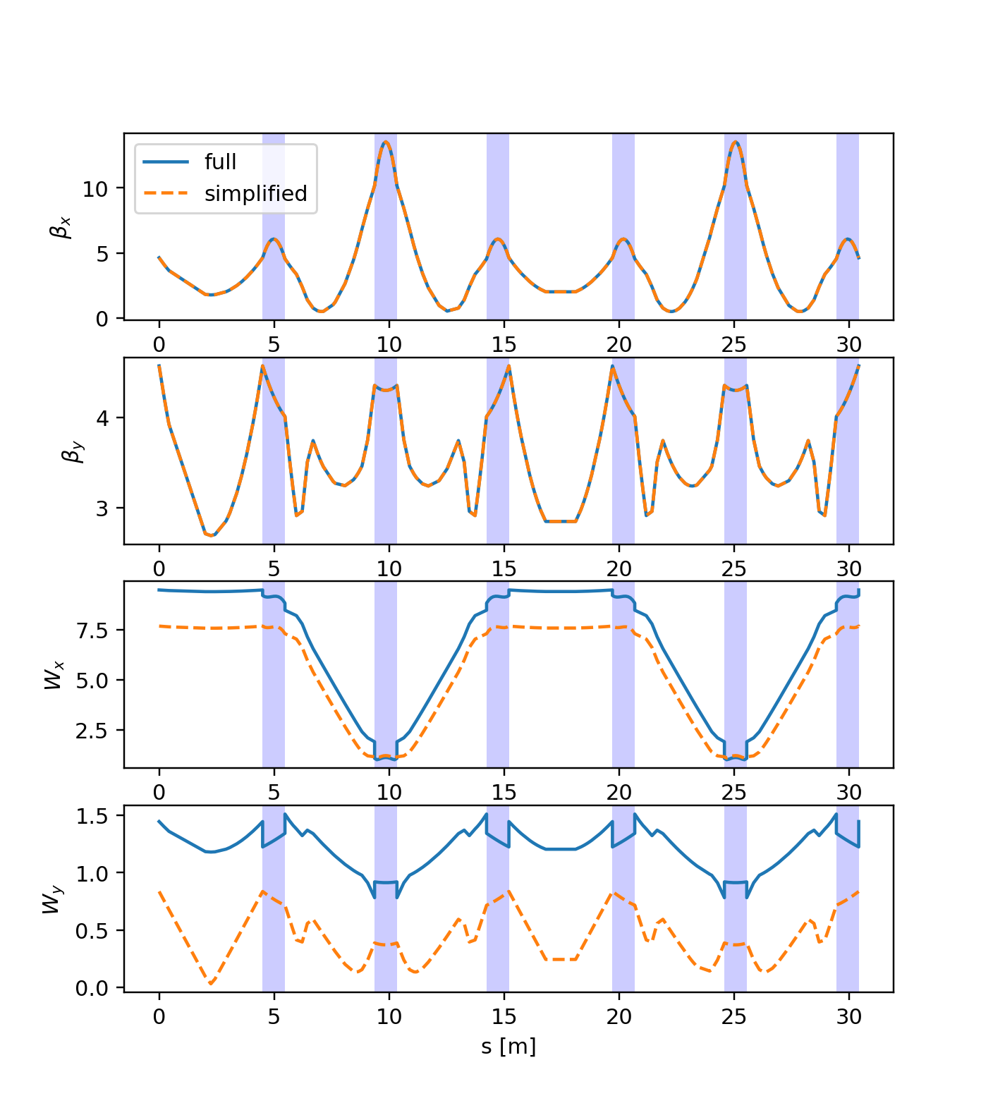
Comparison of the simplified and full model for the CERN ELENA ring (the six bends of the ring are highlighted in blue). While the linear optics is well reproduced by the simplified model, the chromatic properties differ significantly (in particular, note the effect of the dipole edges).