Modeling s-dependent magnetic fields
Overview
The xtrack.SplineBoris element models a thick magnetic element whose
field varies along the longitudinal coordinate. It is suited to devices such
as undulators, wigglers, fringe field and solenoids, for which a constant multipolar
description is not sufficient.
Internally, particles are tracked using a spatial Boris-like integrator. The
method has second-order convergence in the number of integration steps (the
global discretization error scales as n_steps**-2). Although it is not
strictly symplectic, it preserves phase-space volume and its symplectic deviation
decreases quadratically with the number of integration steps. See the
Spatial Boris Integrator chapter of the
Physics Guide for a description of the algorithm and its
main properties.
Within each element, the longitudinal dependence of the field is represented
by fourth-order polynomials and the Lorentz force is integrated with a Boris
stepper. The field data are provided through xtrack.Spline4 objects.
Each object stores the field value and longitudinal derivative at both ends of
an interval, together with its mean value. The bx and by arguments can
also contain tuples of Spline4 objects describing successive transverse
derivatives of the field.
The reconstruction of the three-dimensional field from these on-axis data is
described in the Field expansion for s-dependent magnetic field chapter
of the Physics Guide.
An extended field map is typically represented by a line containing several
SplineBoris elements, with one element for each longitudinal region over
which a polynomial representation is used. The n_steps parameter controls
the number of Boris integration steps within each element.
Building an undulator from a field map
The following example loads a three-dimensional field map of an SLS undulator
and fits the on-axis field and its transverse derivatives in consecutive
longitudinal regions. Each fitted region is converted to a SplineBoris
element. Thin correctors are then inserted near the ends of the resulting line
and matched to close the trajectory through the device.
The FieldFitter used here is an example-specific helper. Users can apply
their own fitting procedure to produce the corresponding Spline4 data for
each longitudinal region.
import xtrack as xt
import pandas as pd

#################################################
# Polynomial fit on the data from the field map #
#################################################

# Load the raw field map data from shared test_data
field_map_path = "../../test_data/sls/undulator_field_map.txt"
df_raw_data = pd.read_csv(
    field_map_path,
    sep=r"\s+",
    header=None,
    names=["X", "Y", "Z", "Bskew", "Bnorm", "Bs"],
).set_index(["X", "Y", "Z"])

# Use fitting procedure to extract field and derivatives on the reference trajectory.
# This class is taylored for this example data, use your own fitting procedure
# for other datasets.
from xtrack._temp.splineboris.field_fitter import FieldFitter
field_fitter = FieldFitter(
    raw_data=df_raw_data,
    xy_point=(0, 0),
    distance_unit=0.001, # dataset uses mm
    min_region_size=10,
    deg=2,
)
spline_data = field_fitter.get_spline_data()

# `spline_data` contains for each longitudinal interval the 4th-order
# polynomial coefficients (in the form of value at start/end of interval,
# longitudinal derivative at start/end of interval, and mean value) for the field
# components and their transverse derivatives. For example:
# spline_data[0] is:
# {'s_start': -1.1,
#  's_end': -1.095,
#  'idx_start': 0,
#  'idx_end': 5,
#  'bs':
#      Spline4(val_start=0.0, der_start=0.0, val_end=0.0, der_end=0.0, mean=0.0),
#  'bx': (
#         # bx on axis (x=0,y=0)
#         Spline4(val_start=0.0002597788559479, der_start=0.003908159160349505,
#                 val_end=0.00027929455770183206, der_end=0.00389142774801777,
#                 mean=0.00026954160840155075),
#         # d bx/d x on axis (x=0,y=0)
#         Spline4(val_start=0.0, der_start=0.0, val_end=0.0, der_end=0.0, mean=0.0),
#         # d^2 bx/d x^2 on axis (x=0,y=0)
#         Spline4(val_start=-0.03587500889997759, der_start=-42.00397475010047,
#                 val_end=-0.04413421209996192, der_end=-6.919120799986231,
#                 mean=-0.04245506171996625)
#        ),
#  'by': (
#       # by on axis (x=0,y=0)
#       Spline4(val_start=0.0020494067017488, der_start=0.0627448571810936,
#               val_end=0.0023965826590473483, der_end=0.07647819250243666,
#               mean=0.0022172898542134225),
#       # d by/d x on axis (x=0,y=0)
#       Spline4(val_start=0.0, der_start=0.0, val_end=0.0, der_end=0.0, mean=0.0),
#       # d^2 by/d x^2 on axis (x=0,y=0)
#       Spline4(val_start=-0.5104028836997457, der_start=-29.057401352068492,
#               val_end=-0.6429682228011369, der_end=-48.71395930245775,
#               mean=-0.5725836650301926)
#      )
# }

#######################################
# Build Xsuite model of the undulator #
#######################################

env = xt.Environment()
env.set_particle_ref('positron', p0c=2.7e9)

# Build and register the SplineBoris elements explicitly.
undulator_element_names = []
for ii, piece in enumerate(spline_data):
    element_name = f'undulator_splineboris_{ii}'

    # Match the field-map resolution: one Boris step per interval
    # between adjacent data points in this piece.
    nn_steps = max(1, piece['idx_end'] - piece['idx_start'])

    env.elements[element_name] = xt.SplineBoris(
        length=piece['s_end'] - piece['s_start'],
        n_steps=nn_steps,
        bs=piece['bs'],
        bx=piece['bx'],
        by=piece['by'],
    )
    undulator_element_names.append(element_name)

undulator = env.new_line(components=undulator_element_names)

###########################################################################
# Install thin dipole correctors at the edges of the undulator to control #
# trajectory along the undulator.                                         #
###########################################################################

# Knobs controlling the correctors
env['k0l_corr1'] = 0.
env['k0l_corr2'] = 0.
env['k0l_corr3'] = 0.
env['k0l_corr4'] = 0.
env['k0sl_corr1'] = 0.
env['k0sl_corr2'] = 0.
env['k0sl_corr3'] = 0.
env['k0sl_corr4'] = 0.

# Create correcto elements
env.new('corr1', xt.Multipole, knl=['k0l_corr1'], ksl=['k0sl_corr1'])
env.new('corr2', xt.Multipole, knl=['k0l_corr2'], ksl=['k0sl_corr2'])
env.new('corr3', xt.Multipole, knl=['k0l_corr3'], ksl=['k0sl_corr3'])
env.new('corr4', xt.Multipole, knl=['k0l_corr4'], ksl=['k0sl_corr4'])

# Insert correctors
l_undulator = undulator.get_length()
undulator.insert([
    env.place('corr1', at=0.02),
    env.place('corr2', at=0.1),
    env.place('corr3', at=l_undulator - 0.1),
    env.place('corr4', at=l_undulator - 0.02),
], s_tol=5e-3) # large s_tol avoids slicing the SplineBoris elements

# Use optimizer to control the orbit
opt = undulator.match(
    solve=False,
    betx=1, bety=1,
    include_collective=True,
    vary=xt.VaryList(['k0l_corr1', 'k0sl_corr1',
                      'k0l_corr2', 'k0sl_corr2',
                      'k0l_corr3', 'k0sl_corr3',
                      'k0l_corr4', 'k0sl_corr4',
                      ], step=1e-6),
    targets=[
        xt.TargetSet(x=0, px=0, y=0, py=0., at=xt.END),
        xt.TargetSet(x=0., y=0, at='corr2'),
        xt.TargetSet(x=0., y=0, at='corr3')
        ],
)
opt.solve()

###############################
# Save undulator to json file #
###############################

undulator.to_json('sls_undulator.json')

##################################
# Plot orbit along the undulator #
##################################

import matplotlib.pyplot as plt

tw_undulator = undulator.twiss4d(betx=1, bety=1)

fig_orbit = plt.figure(1, figsize=(10, 6))
tw_undulator.plot('x y', figure=fig_orbit)
fig_orbit.savefig('splineboris_undulator_trajectory.png', dpi=200,
                  bbox_inches='tight')

plt.show()

# Complete source: xtrack/examples/splineboris/004a_build_undulator.py
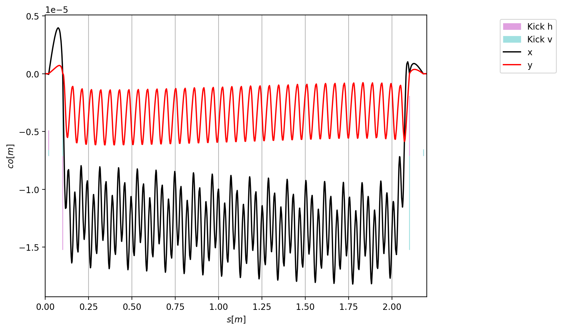
Horizontal and vertical trajectories through the corrected undulator.
Installing the undulator in a ring
A line made of SplineBoris elements can be serialized and imported into
another xtrack.Environment. In the following example, the undulator
built above is loaded, installed at several straight sections of the SLS ring,
and included in a four-dimensional Twiss calculation.
import xtrack as xt
import matplotlib.pyplot as plt

# Load the SLS ring
madx_file = '../../test_data/sls/sls.madx'
env = xt.load(str(madx_file))
line_sls = env.lines['ring']
line_sls.set_particle_ref('positron', p0c=2.7e9)
tt = line_sls.get_table()

# Import the undulator in the environment containing the ring
undulator = xt.load('./sls_undulator.json')
env.import_line(undulator, line_name='undulator')

# Install the undulator at several locations in the ring
wiggler_places = [
    'ars02_uind_0500_1',
    'ars03_uind_0380_1',
    'ars04_uind_0500_1',
    'ars05_uind_0650_1',
    'ars06_uind_0500_1',
    'ars07_uind_0200_1',
    'ars08_uind_0500_1',
    'ars09_uind_0790_1',
    'ars11_uind_0210_1',
    'ars11_uind_0610_1',
    'ars12_uind_0500_1',
]
insertions = []
for wig_place in wiggler_places:
    insertions.append(
        env.place(env['undulator'], anchor='start', at=tt['s_start', wig_place]))
line_sls.insert(insertions)

# Twiss with undulators
tw = line_sls.twiss4d()

# Plot and save the closed orbit
fig_closed_orbit = plt.figure(1, figsize=(10, 6))
tw.plot('x y', figure=fig_closed_orbit)
fig_closed_orbit.savefig('splineboris_sls_closed_orbit.png', dpi=200,
                         bbox_inches='tight')

# Complete source: xtrack/examples/splineboris/004b_undulators_in_sls_ring.py
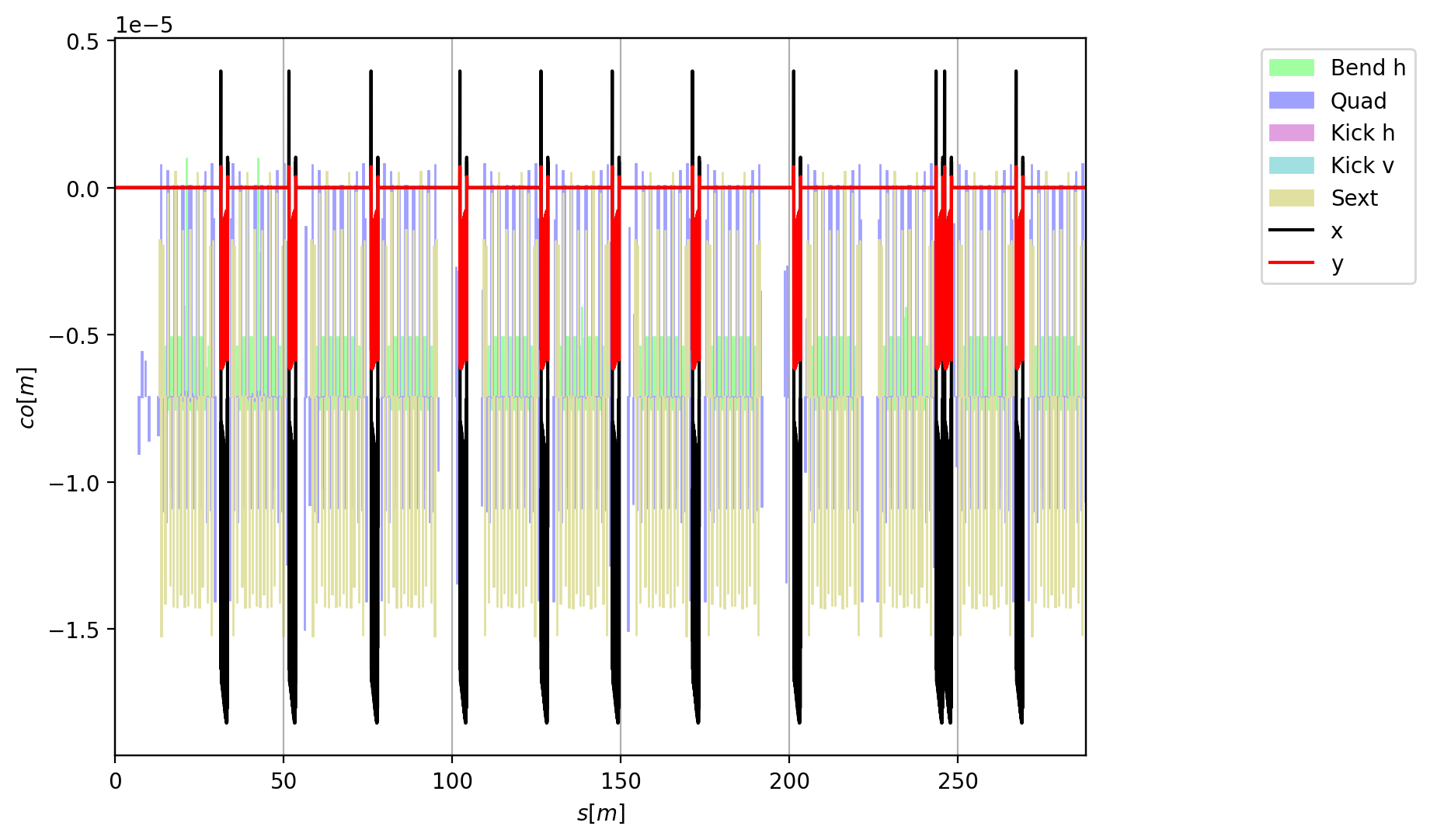
Horizontal and vertical closed orbit in the SLS ring with the undulators installed.