Particle-matter interaction and collimation
Introduction
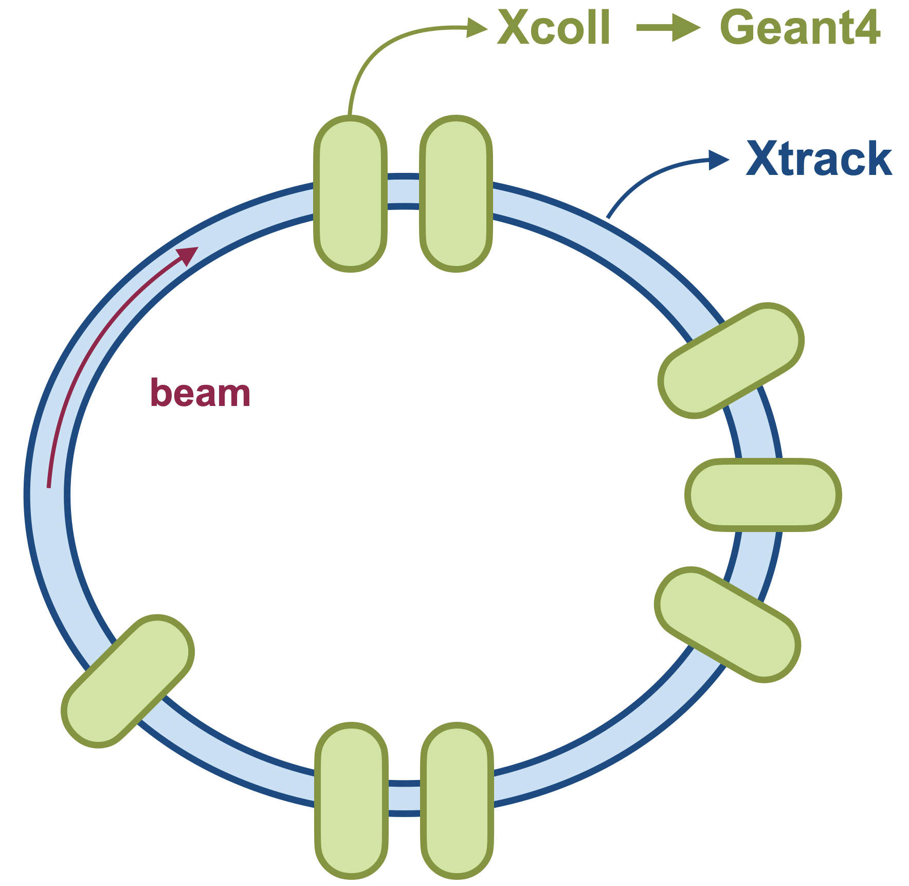
In Xsuite, collimation is added to the simulations by the Xcoll package.
The collimators themselves are created as instances of xcoll.EverestCollimator, xcoll.EverestCrystal and xcoll.BlackAbsorber. In addition, we also have xcoll.EverestBlock. The Xcoll package also describes the interaction between the particles and the collimators in the simulation.
Loss maps are created after the simulations to assess the performance of the LHC collimation system. They give information about where the beam losses are located in the LHC. The loss map, after one simulation, is created as an instance of xcoll.LossMap.
Collimator objects
BaseCollimator
Since xcoll.EverestCollimator, xcoll.EverestCrystal and xcoll.BlackAbsorber describes different kinds of collimators they all inherit from the abstract class BaseCollimator which contains all the basic attributes of a collimator. Some of these attributes, or fields, are made accessible to the C tracking code as seen in the code block below.
class BaseCollimator(xt.BeamElement):
    _xofields = {
        'inactive_front': xo.Float64,  # Drift before jaws
        'active_length':  xo.Float64,  # Length of jaws
        'inactive_back':  xo.Float64,  # Drift after jaws
        'jaw_L':          xo.Float64,  # left jaw (distance to ref)
        'jaw_R':          xo.Float64,  # right jaw
        'ref_x':          xo.Float64,  # center of collimator reference frame
        'ref_y':          xo.Float64,
        'sin_zL':         xo.Float64,  # angle of left jaw
        'cos_zL':         xo.Float64,
        'sin_zR':         xo.Float64,  # angle of right jaw
        'cos_zR':         xo.Float64,
        'sin_yL':         xo.Float64,  # tilt of left jaw (around jaw midpoint)
        'cos_yL':         xo.Float64,
        'tan_yL':         xo.Float64,
        'sin_yR':         xo.Float64,  # tilt of right jaw (around jaw midpoint)
        'cos_yR':         xo.Float64,
        'tan_yR':         xo.Float64,
        '_side':          xo.Int8,     # is it a onesided collimator?
        'active':         xo.Int8
    }
However, to make things more user-friendly the BaseCollimator has more properties defined in the class itself. These properties uses the fields from the code block above to define properties such as jaw_LU(), angle() and tilt().
The collimator jaws are separated into the left and the right jaw, as seen defined in the code block above as well. In the figure below, you can see how ‘jaw_L’ and ‘jaw_R’ are defined. However, sometimes it is necessary to know, or change, the position of the corners of the collimator. The first pair of corners are called jaw_LU() and jaw_RU(), where the ‘U’ stands for upstream. The two remaining corners are defined as jaw_LD() and jaw_RD(), where the ‘D’ stands for downstream. Note that when setting the value of e.g. jaw_RU() then jaw_RD() is kept fixed while both ‘jaw_R’ and the tilt changes.
collimatorObject.jaw
collimatorObject.jaw_LU
collimatorObject.jaw_RU
collimatorObject.jaw_RD
collimatorObject.jaw_RU


In addition, it is convenient to have the angle and the tilt of the jaws. The angle is the angle of the tilt of the jaws in the xy-plane while the tilt is the angle of the tilt of the jaws in the x’z-plane. For clarity, the angle is shown as alpha, and the tilt as theta in the images. Note that the tilt is in radians while the angle is in degrees.
collimatorObject.angle
collimatorObject.angle_L
collimatorObject.angle_R
collimatorObject.tilt
collimatorObject.tilt_L
collimatorObject.tilt_R
Furthermore, it is also possible to get (and set) the length and the side of the collimator.
collimatorObject.side
collimatorObject.length
EverestCollimator
The EverestCollimator contains all the same fields as BaseCollimator, but in addition it also has these:
class EverestCollimator(BaseCollimator):
 _xofields = { **BaseCollimator._xofields,
     '_material':        Material,
     'rutherford_rng':   xt.RandomRutherford,
     '_tracking':        xo.Int8
 }
The new field of interest for the user is the material of the collimator. This is accessed by the method EverestCollimator.material(). The material itself is an instance of xcoll.materials.Material.
EverestCrystal
EverestCrystal has the same fields as BaseCollimator, but in addition it has some extra fields which are needed to describe the crystal collimator. Note also that the material used for the crystal collimator is not the same as for xcoll.EverestCollimator, but an instance of xcoll.materials.CrystalMaterial.
class EverestCrystal(BaseCollimator):
    _xofields = { **BaseCollimator._xofields,
        'align_angle':        xo.Float64,  #  = - sqrt(eps/beta)*alpha*nsigma
        '_bending_radius':    xo.Float64,
        '_bending_angle':     xo.Float64,
        '_critical_angle':    xo.Float64,
        'xdim':               xo.Float64,
        'ydim':               xo.Float64,
        'thick':              xo.Float64,
        'miscut':             xo.Float64,
        '_orient':            xo.Int8,
        '_material':          CrystalMaterial,
        'rutherford_rng':     xt.RandomRutherford,
        '_tracking':          xo.Int8
    }
These new fields are accessed through the methods:
EverestCrystal.critical_angle
EverestCrystal.bending_radius
EverestCrystal.bending_angle
EverestCrystal.material
EverestCrystal.lattice
BlackAbsorber
xcoll.BlackAbsorber is different from xcoll.EverestCollimator and EverestCrystal. The absorber has only one extra field compared to the xcoll.BaseCollimator:
class BlackAbsorber(BaseCollimator):
    _xofields = { **BaseCollimator._xofields,
        '_tracking':        xo.Int8
    }
BaseBlock and EverestBlock
xcoll.EverestBlock, which inherit xcoll.BaseBlock, describes a block with an infinite transversal length. This class has the fields:
class EverestBlock(BaseBlock):
 _xofields = { **BaseBlock._xofields,
     '_material':        Material,
     'rutherford_rng':   xt.RandomRutherford,
     '_tracking':        xo.Int8,
     '_only_mcs':        xo.Int8
 }
Furthermore, xcoll.EverestBlock needs a material, which is an instance of xcoll.materials.Material, and that can be accessed through
EverestBlock.material
Creating a Collimator or Block object
A collimator (or block) object can be created in two different ways; either directly with the class or by loading from file. For example:
import xcoll as xc

block = xc.EverestBlock(length=1., material=xc.materials.Tungsten)
collimator = xc.EverestCollimator(length=1., material=xc.materials.Tungsten)
collimator_crystal = xc.EverestCrystal(length=1., material=xc.materials.SiliconCrystal)
black_absorber = xc.BlackAbsorber(length=1., material=xc.materials.Graphite)
Or, by using the CollimationManager to load from file:
path_in  = xc._pkg_root.parent / 'examples'
coll_manager = xc.CollimatorManager.from_yaml(path_in / 'colldb' / f'lhc_run3.yaml',
                                           line=line, beam=beam, _context=context)

# Install collimators in line as black absorbers
coll_manager.install_everest_collimators(verbose=True)
Generating particles on a collimator
For some collimation studies it is convenient to generate a initial pencil distribution on a collimator. Xcoll has its own function for this xcoll.generate_pencil_on_collimator(). An example is shown below.
import xcoll as xc
import xpart as xp
import xtrack as xt
import numpy as np
import json

beam =  1
plane = 'H'
num_turns     = 200
num_particles = 10000
path_in  = xc._pkg_root.parent / 'examples'

# Load from json
with open(os.devnull, 'w') as fid:
   with contextlib.redirect_stdout(fid):
        line = xt.Line.from_json(path_in / 'machines' / f'lhc_run3_b{beam}.json')

# Initialise collmanager
coll_manager = xc.CollimatorManager.from_yaml(path_in / 'colldb' / f'lhc_run3.yaml',
                                      line=line, beam=beam, _context=context)
# Install collimators into line
coll_manager.install_everest_collimators(verbose=True)

# Aperture model check
print('\nAperture model check after introducing collimators:')
with open(os.devnull, 'w') as fid:
    with contextlib.redirect_stdout(fid):
        df_with_coll = line.check_aperture()
assert not np.any(df_with_coll.has_aperture_problem)


# Build the tracker
coll_manager.build_tracker()
# Set openings
coll_manager.set_openings()

tcp  = f"tcp.{'c' if plane=='H' else 'd'}6{'l' if int(beam)==1 else 'r'}7.b{beam}"
emittance = coll_manager.colldb.emittance
beta_gamma_rel = coll_manager.colldb._beta_gamma_rel
part = xc.generate_pencil_on_collimator(line=line, emittance=emittance, beta_gamma_rel=bet,
                                      collimator_name=tcp, num_particles=num_particles)
Lossmaps
Lossmaps are created as instances of xcoll.LossMap. The lossmap itself and its summary are calculated when the object is created. It is also possible to save both the lossmap and summary to file with xcoll.LossMap.to_json() and xcoll.LossMap.save_summary(). For example:
Loss location refinement
In Xtrack simulations particles are lost at defined aperture elements (e.g.
xtrack.LimitRect, xtrack.LimitEllipse, xtrack.LimitRectEllipse,
xtrack.LimitPolygon). A more accurate estimate of the loss locations can be
obtained after the tracking is finished using the
xtrack.LossLocationRefinement tool . The tool builds
an interpolated aperture model between the aperture elements and backtracks the
particles in order to identify the impact point. The following example illustrates
how to use this feature.
See also: xtrack.LossLocationRefinement
import numpy as np

import xtrack as xt
import xobjects as xo


###################
# Build test line #
###################

# We build a test line having two aperture elements which are shifted and
# rotated w.r.t. the accelerator reference frame.

# Define aper_0
aper_0 = xt.LimitEllipse(a=2e-2, b=1e-2)
shift_aper_0 = (1e-2, 0.5e-2)
rot_deg_aper_0 = 10.

# Define aper_1
aper_1 = xt.LimitRect(min_x=-1e-2, max_x=1e-2,
                      min_y=-2e-2, max_y=2e-2)
shift_aper_1 = (-5e-3, 1e-2)
rot_deg_aper_1 = 10.
aper_1.shift_x = shift_aper_1[0]
aper_1.shift_y = shift_aper_1[1]
aper_1.rot_s_rad = np.deg2rad(rot_deg_aper_1)


# aper_0_sandwitch
line_aper_0 = xt.Line(
    elements=[xt.Translation(shift_x=shift_aper_0[0], shift_y=shift_aper_0[1]),
              xt.Rotation(rot_s_rad=np.deg2rad(rot_deg_aper_0)),
              aper_0,
              xt.Multipole(knl=[0.001]),
              xt.Rotation(rot_s_rad=-np.deg2rad(rot_deg_aper_0)),
              xt.Translation(shift_x=-shift_aper_0[0], shift_y=-shift_aper_0[1])])

# aper_1_sandwitch
line_aper_1 = xt.Line(
    elements=[aper_1,
              xt.Multipole(knl=[0.001])
        ])

#################
# Build tracker #
#################

line=xt.Line(
    elements = ((xt.Drift(length=0.5),)
                + line_aper_0.elements
                + (xt.Drift(length=1),
                   xt.Drift(length=1),
                   xt.Drift(length=1.),)
                + line_aper_1.elements))
num_elements = len(line.element_names)

# Generate test particles
particles = xt.Particles(px=np.random.uniform(-0.01, 0.01, 10000),
                         py=np.random.uniform(-0.01, 0.01, 10000))

#########
# Track #
#########

line.track(particles)

########################
# Refine loss location #
########################

loss_loc_refinement = xt.LossLocationRefinement(line,
        n_theta = 360, # Angular resolution in the polygonal approximation of the aperture
        r_max = 0.5, # Maximum transverse aperture in m
        dr = 50e-6, # Transverse loss refinement accuracy [m]
        ds = 0.1, # Longitudinal loss refinement accuracy [m]
        save_refine_lines=True # Diagnostics flag
        )


loss_loc_refinement.refine_loss_location(particles)


# Complete source: xtrack/examples/collimation/001_loss_location_refinement.py
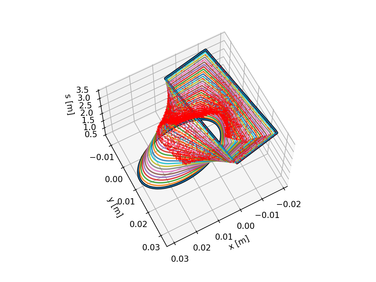
Generated transition between the defined apertures. Red dots represent the location of the particle-loss events. See the code generating the image.
Material definitions
Materials database
Xcoll ships with a built-in database of materials (which cannot be modified at runtime):
import xcoll as xc
xc.materials.show(full=True)
Materials can be accessed from the module by their full name only:
print(xc.materials.Aluminium)
or from the database using their name or aliases:
mat1 = xc.materials.db['Aluminium']
mat2 = xc.materials.db['Aluminum']
mat3 = xc.materials.db['Al']
print(mat1)
print(mat2)
print(mat3)
print(mat1 == mat2)
print(mat1 == mat3)
Note that the collimators in the LHC are made of CFC (xc.materials.CarbonFibreCarbon) and not just
plain carbon (as it is colloquially named). Hence, refrain from using (xc.materials.Carbon) as a
collimator material (unless this is the explicit purpose), as it does not yet support full Everest
scattering (see below).
When a material is known to FLUKA or Geant4, it has a fluka_name resp geant4_name attribute:
print(f"Copper-Diamond in FLUKA is called: {xc.materials.CopperDiamond.fluka_name}")
print(f"Aluminium in Geant4 is called: {mat1.geant4_name}")
Defining New Materials
All elements in the periodic table are predefined in the database.
When defining a new elemental material (i.e. an allotrope), the fields
'Z', 'A', and 'density' are required:
It is not possible to redefine existing elements in the database, but it is possible to adapt them with the adapt method.
Ozone = xc.materials.Oxygen.adapt(density=2.144e-3, name='Ozone',
                                  info="O3, but defined as element instead of compound.")
When adapting a material, unspecified fields are taken from the original material, like the state, and temperature and pressure at which the density applies:
print(xc.materials.Oxygen)
print(Ozone)
print(xc.materials.Oxygen.to_dict())
print(Ozone.to_dict())
# But names and info are not copied:
print(f"Original name: {xc.materials.Oxygen.name}, adapted name: {Ozone.name}")
print(f"Original short name: {xc.materials.Oxygen.short_name}, adapted short name: {Ozone.short_name}")
print(f"Original FLUKA name: {xc.materials.Oxygen.fluka_name}, adapted FLUKA name: {Ozone.fluka_name}")
print(f"Original Geant4 name: {xc.materials.Oxygen.geant4_name}, adapted Geant4 name: {Ozone.geant4_name}")
print(f"Original info: `{xc.materials.Oxygen.info}`")
print(f"Adapted info: `{Ozone.info}`")
Defining New Compounds and Mixtures
Compounds are defined by specifying their components as a chemical formula,
and hence the fields components and n_atoms:
Ethanol = xc.Material(components=['C', 'H', 'O'], n_atoms=[2, 6, 1], density=0.78945, name='Ethanol',
                      state='liquid', temperature=293.15)
print(Ethanol)
print(Ethanol.composition)
# Any doubled components are automatically combined:
EthanolBis = xc.Material(components=['C', 'H', 'C', 'H', 'O', 'H'], n_atoms=[1, 3, 1, 2, 1, 1], density=0.78945,
                name='EthanolBis', state='liquid', temperature=293.15)
print(f"{Ethanol == EthanolBis=}")
Mixtures are not a chemical formula, but a physical mixture of different materials. They are defined by specifying their components and either their mass fractions, volume fractions, or molar fractions:
Concrete = xc.Material(components=['H', 'C', 'O', 'Na', 'Mg', 'Al', 'Si', 'K', 'Ca', 'Fe'],
                       mass_fractions=[0.01, 0.001, 0.529107, 0.016, 0.002, 0.033872, 0.337021, 0.013, 0.044, 0.014],
                       name='Concrete', density=2.35, state='solid')
print(Concrete)
print(Concrete.composition)
print(Concrete.to_dict())
It is possible to combine any previously defined material as components of a mixture (even mixtures themselves). The code will recursively resolve the elemental composition:
Glucose      = xc.Material(components=['C', 'H', 'O'], n_atoms=[6, 12, 6], density=1.54, name='Glucose')
Anethole     = xc.Material(components=['C', 'H', 'O'], n_atoms=[10, 12, 1], density=1.05, name='Anethole',
                        info="Main flavor component (anise) of absinthe.")
components=[Ethanol, xc.materials.Water, Glucose, Anethole]
volume_fractions=[0.7, 0.25, 0.045, 0.005]
FakeAbsinthe = xc.Material(components=components, volume_fractions=volume_fractions,
                        density = sum([vf * el.density for el, vf in zip(components, volume_fractions)]),
                        name='FakeAbsinthe', state='liquid')
print(FakeAbsinthe)
print(FakeAbsinthe.composition)
print(FakeAbsinthe.to_dict())
Everest Compatibility
Not all materials are 100% compatible with Everest. Multiple Coulomb scattering and ionisation loss are
always supported, but nuclear interactions are only supported for materials known to Everest.
This can be checeked with the full_everest_supported attribute:
print(f"CFC full Everest compatibility: {xc.materials.CarbonFibreCarbon.full_everest_supported}")
print(f"Ethanol full Everest compatibility: {Ethanol.full_everest_supported}")
print(f"FakeAbsinthe full Everest compatibility: {FakeAbsinthe.full_everest_supported}")
Beam interaction (generation of secondary particles)
Xtrack includes an interface to ease the modeling of beam-matter interaction (collimators, beam-gas, collisions with another beam), including the loss of the impacting particles and the production of secondary particles, which need to be tracked together with the surviving beam. Such interface can be used to create a link with other programs for the modeling of these effects, e.g. GuineaPig. Note that although this approach was originally used to link Xcoll to Geant4 and FLUKA, these codes are currently linked more directly with dedicated beam elements (see Linking external codes for material Interactions).
The interaction is defined as an object that provides a .interact(particles)
method, which sets to zero or negative the state flag for the particles that are lost and
returns a dictionary with the coordinates of the secondary particles that are
emitted. The interaction process is embedded in one or multiple
xtrack.BeamInteraction beam elements that can be included in Xtrack line.
This is illustrated by the following example:
import numpy as np

import xtrack as xt

######################################
# Create a dummy collimation process #
######################################

class DummyInteractionProcess:
    '''
    I kill some particles. I kick some others by an given angle
    and I generate some secondaries with the opposite angles.
    '''
    def __init__(self, fraction_lost, fraction_secondary, length, kick_x):

        self.fraction_lost = fraction_lost
        self.fraction_secondary = fraction_secondary
        self.kick_x = kick_x
        self.length = length

        self.drift = xt.Drift(length=self.length)


    def interact(self, particles):

        self.drift.track(particles)

        n_part = particles._num_active_particles

        # Kill some particles
        mask_kill = np.random.uniform(size=n_part) < self.fraction_lost
        particles.state[:n_part][mask_kill] = -1 # special flag`


        # Generate some more particles
        mask_secondary = np.random.uniform(size=n_part) < self.fraction_secondary
        n_products = np.sum(mask_secondary)
        if n_products>0:
            products = {
                's': particles.s[:n_part][mask_secondary],
                'x': particles.x[:n_part][mask_secondary],
                'px': particles.px[:n_part][mask_secondary] + self.kick_x,
                'y': particles.y[:n_part][mask_secondary],
                'py': particles.py[:n_part][mask_secondary],
                'zeta': particles.zeta[:n_part][mask_secondary],
                'delta': particles.delta[:n_part][mask_secondary],

                'mass_ratio': particles.x[:n_part][mask_secondary] *0 + 1.,
                'charge_ratio': particles.x[:n_part][mask_secondary] *0 + 1.,

                'parent_particle_id': particles.particle_id[:n_part][mask_secondary],
                'at_element': particles.at_element[:n_part][mask_secondary],
                'at_turn': particles.at_turn[:n_part][mask_secondary],
                }
        else:
            products = None

        return products

############################################################
# Create a beam interaction from the process defined above #
############################################################

interaction_process=DummyInteractionProcess(length=1., kick_x=4e-3,
                                            fraction_lost=0.0,
                                            fraction_secondary=0.2)
collimator = xt.BeamInteraction(length=interaction_process.length,
                                      interaction_process=interaction_process)

########################################################
# Create a line including the collimator defined above #
########################################################

line = xt.Line(elements=[
    xt.Multipole(knl=[0,0]),
    xt.LimitEllipse(a=2e-2, b=2e-2),
    xt.Drift(length=1.),
    xt.Multipole(knl=[0,0]),
    xt.LimitEllipse(a=2e-2, b=2e-2),
    xt.Drift(length=2.),
    collimator,
    xt.Multipole(knl=[0,0]),
    xt.LimitEllipse(a=2e-2, b=2e-2),
    xt.Drift(length=10.),
    xt.LimitEllipse(a=2e-2, b=2e-2),
    xt.Drift(length=10.),
    ])

line.config.XTRACK_GLOBAL_XY_LIMIT = 1e3

##########################
# Build particles object #
##########################

# We prepare empty slots to store the product particles that will be
# generated during the tracking.
particles = xt.Particles(
        _capacity=200000,
        x=np.zeros(100000))

#########
# Track #
#########

line.track(particles)

############################
# Loss location refinement #
############################

loss_loc_refinement = xt.LossLocationRefinement(line,
                                            n_theta = 360,
                                            r_max = 0.5, # m
                                            dr = 50e-6,
                                            ds = 0.05,
                                            save_refine_lines=True)

loss_loc_refinement.refine_loss_location(particles)


# Complete source: xtrack/examples/collimation/003_all_together.py
Linking external codes for material Interactions
Xcoll’s internal material interaction model Everest is adequate for simulating
proton beams. In this model, no secondary particles are generated, and scattering
processes are modelled semi-continously to limit computation time. In case one is
performing simulations with heavy ions or electrons, where the production of secondary
particles becomes important as they could survive significant distances in the
accelerator, or if one requires a more accurate description of the scattering processes,
it is advisable to link Xcoll to an external material interaction code that supports
all particle types and performs a stepwise integration of the scattering processes.
In doing so, tracking is performed in Xsuite as usual but when a particle enters a material block or collimator, its coordinates and momenta are passed to the external code, which then performs the tracking through the material block, including the generation of secondary particles. After exiting the material block, the updated coordinates and momenta of the primary and secondary particles are passed back to Xsuite for further tracking.
Managing the connection: the Engine
Managing the external code, both its execution and the communication with Xcoll/Xsuite,
is handled by a dedicated Engine in Xcoll. This engine is responsible for
launching the external code, defining the physics parameters to be considered, sending
and retrieving the particle data, and cleaning up after the simulation. The main methods
of the engine are:
Engine.start(line=None, elements=None, names=None, input_file=None, cwd=None,
             clean=True, **kwargs)

Engine.stop(clean=False)
To start the engine, there are multiple options:
Engine.start(line=line): the engine will link all relevant elements in the line
Engine.start(line=line, names=names): the engine will only link the elementsnames(which should be present in the line)
Engine.start(elements=elements): the engine will link the provided list of elements
Engine.start(..., input_file=input_file): the engine will use the provided input file instead of auto-generating one (its elements need to match those provided)
It is possible to specify the working directory cwd where the external code will be executed and where input/output files and logs will be stored.
If clean=True, the working directory will be cleaned up.
If more control over the input file is desired, it is possible to pre-generate it on a list of elements using:
Engine.generate_input_file(line=None, elements=None, names=None, filename=None, clean=True, **kwargs)
such that it can be manually modified before starting the engine with it.
There are many arguments that can be passed to the engine when starting it, or when generating the input file.
Furthermore, these arguments can also be set as attributes of the engine before starting it.
The difference lies in the fact that arguments passed to the start() or generate_input_file()
methods will only be used for that specific call, while attributes set on the engine will persist
for future calls as well.
The following options can be set:
particle_ref: xpart.Particles  # Required
seed: int64                    # optional (default None)
verbose: bool                  # optional (default False)
input_file: str | Path         # optional (default None)
return_all: bool               # optional (default None)
return_none: bool              # optional (default None)
return_leptons: bool           # optional (default False)
return_mesons: bool            # optional (default False)
return_exotics: bool           # optional (default False)
return_baryons: bool           # optional (default False)
return_neutral: bool           # optional (default False)
return_photons: bool           # optional (default False)
return_electrons: bool         # optional (default True)
return_muons: bool             # optional (default True)
return_tauons: bool            # optional (default False)
return_neutrinos: bool         # optional (default False)
return_protons: bool           # optional (default True)
return_neutrons: bool          # optional (default False)
return_ions: bool              # optional (default True)
The return flags can be combined arbitrarily to select which particle types should be
returned to Xsuite after the interaction. In particular, return_none and return_all
can be used to specify only a few particles that will resp. won’t be returned.
Note that it is important that only one instance of the engine is active at any
given time, as multiple instances could lead to conflicts in the communication with
the external code. Therefore, one should never directly call any Engine (like
Geant4Engine(...)). Instead, for each external code there is a dedicated engine
instantiated at Xcoll import time, which can be accessed directly on the package. For
instance, the Geant4 engine is accessed as xcoll.geant4.engine.
Geant4 via BDSIM
To use Geant4 as external code for material interactions in Xcoll, we use the Beam Delivery SIMulation (BDSIM), which is a Geant4-based particle interaction code, which wraps around Geant4 and is specifically designed for accelerator applications. To link Xcoll to BDSIM/Geant4, a full installation of both is required. The easiest way to install BDSIM is via Conda/Mamba. After installing Conda, one can create a dedicated environment for BDSIM/Geant4 and install it via:
mamba create -n bdsim -c conda-forge bdsim-g4
conda activate bdsim
Running an Xcoll simulation is, after installing BDSIM/Geant4, straightforward. Below is an example snippet where a Geant4 collimator is created and linked to the Geant4 engine in Xcoll:
import xtrack as xt
import xpart as xp
import xcoll as xc

num_part = 10000
capacity = num_part*10  # allocate extra capacity for secondaries

coll = xc.Geant4Collimator(length=0.4, material='MoGR')
coll.jaw = 0.001

# Connect to Geant4
xc.geant4.engine.particle_ref = xt.Particles('Pb208', p0c=6.8e12*82)
xc.geant4.engine.start(elements=coll, relative_energy_cut=1e-3, return_all=True, clean=True, verbose=False)

x_init   = np.random.normal(loc=0.002, scale=0.2e-3, size=num_part)
part_init = xp.build_particles(x=x_init, particle_ref=xc.geant4.engine.particle_ref,
                               _capacity=capacity)
part = part_init.copy()

# Do the tracking in Geant4
coll.track(part)

# stop the engine
xc.geant4.engine.stop()

# Print out the results
mask = (part.state > 0) | (part.particle_id >= num_part)
pdg_ids = np.unique(part.pdg_id[mask], return_counts=True)
idx = np.argsort(pdg_ids[1])[::-1]
print(f"Returned {np.sum(mask)} particles ({np.sum(part.particle_id >= num_part)} secondaries):")
for pdg_id, num in zip(pdg_ids[0][idx], pdg_ids[1][idx]):
    try:
        name = pdg.get_name_from_pdg_id(pdg_id, long_name=False)
    except ValueError:
        name = 'unknown'
    print(f"  {num:6} {name:12}   (PDG ID: {pdg_id:5})")
More examples can be found in the Xcoll examples repository.