Tune footprint and stability diagram
The Line class provides a method to compute and optionally plot the tune footprint as illustrated in the following example.
Basic usage
See also: xtrack.Line.get_footprint()
import numpy as np

import xtrack as xt

import matplotlib.pyplot as plt

nemitt_x = 1e-6
nemitt_y = 1e-6


line = xt.load(
    '../../test_data/hllhc15_noerrors_nobb/line_w_knobs_and_particle.json')
line.set_particle_ref('proton', p0c=7e12)

plt.close('all')
plt.figure(1)

# Compute and plot footprint
fp0 = line.get_footprint(nemitt_x=nemitt_x, nemitt_y=nemitt_y)
fp0.plot(color='k', label='I_oct=0')

# Change octupoles strength and compute footprint again
line['i_oct_b1'] = 500
fp1 = line.get_footprint(nemitt_x=nemitt_x, nemitt_y=nemitt_y)
fp1.plot(color='r', label='I_oct=500')

# Change octupoles strength and compute footprint again
line['i_oct_b1'] = -250
fp2 = line.get_footprint(nemitt_x=nemitt_x, nemitt_y=nemitt_y)
fp2.plot(color='b', label='I_oct=-250')

plt.legend()

plt.figure(2)

line['i_oct_b1'] = 0
fp0_jgrid = line.get_footprint(nemitt_x=nemitt_x, nemitt_y=nemitt_y,
                         mode='uniform_action_grid')
fp0_jgrid.plot(color='k', label='I_oct=0')

# Change octupoles strength and compute footprint again
line['i_oct_b1'] = 500
fp1_jgrid = line.get_footprint(nemitt_x=nemitt_x, nemitt_y=nemitt_y,
                            mode='uniform_action_grid')
fp1_jgrid.plot(color='r', label='I_oct=500')

# Change octupoles strength and compute footprint again
line['i_oct_b1'] = -250
fp2_jgrid = line.get_footprint(nemitt_x=nemitt_x, nemitt_y=nemitt_y,
                         mode='uniform_action_grid')
fp2_jgrid.plot(color='b', label='I_oct=-250')

plt.legend()
plt.show()

# Complete source: xtrack/examples/footprint/000_footprint.py
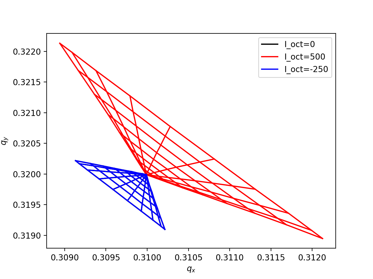
Footprints produced with a polar grid.
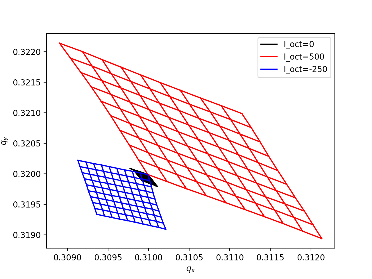
Footprints produced with a uniform grid in action space.
Linear rescale on knobs
In some cases the effects introducing the detuning also introduce other effects (e.g. coupling, or non-linear resonances) that disturb the particles tune measurement. In this case it is possible to rescale quantify the detuning for smaller values of the knobs associate to the detuning effects and rescale to the actual value of the knob. This can be done by the linear_rescale_on_knobs option as illustrated in the following example for a case where the detuning with amplitude is introduced by beam-beam interactions.
See also: xtrack.Line.get_footprint()
import xtrack as xt

collider = xt.load('./collider_04_tuned_and_leveled_bb_on.json')

fp_polar_no_rescale = collider['lhcb1'].get_footprint(nemitt_x=2.5e-6, nemitt_y=2.5e-6)

fp_polar_with_rescale = collider['lhcb1'].get_footprint(
    nemitt_x=2.5e-6, nemitt_y=2.5e-6,
    linear_rescale_on_knobs=[
        xt.LinearRescale(knob_name='beambeam_scale', v0=0.0, dv=0.1)]
    )

# Complete source: xmask/examples/hllhc15_collision/005_footprint.py
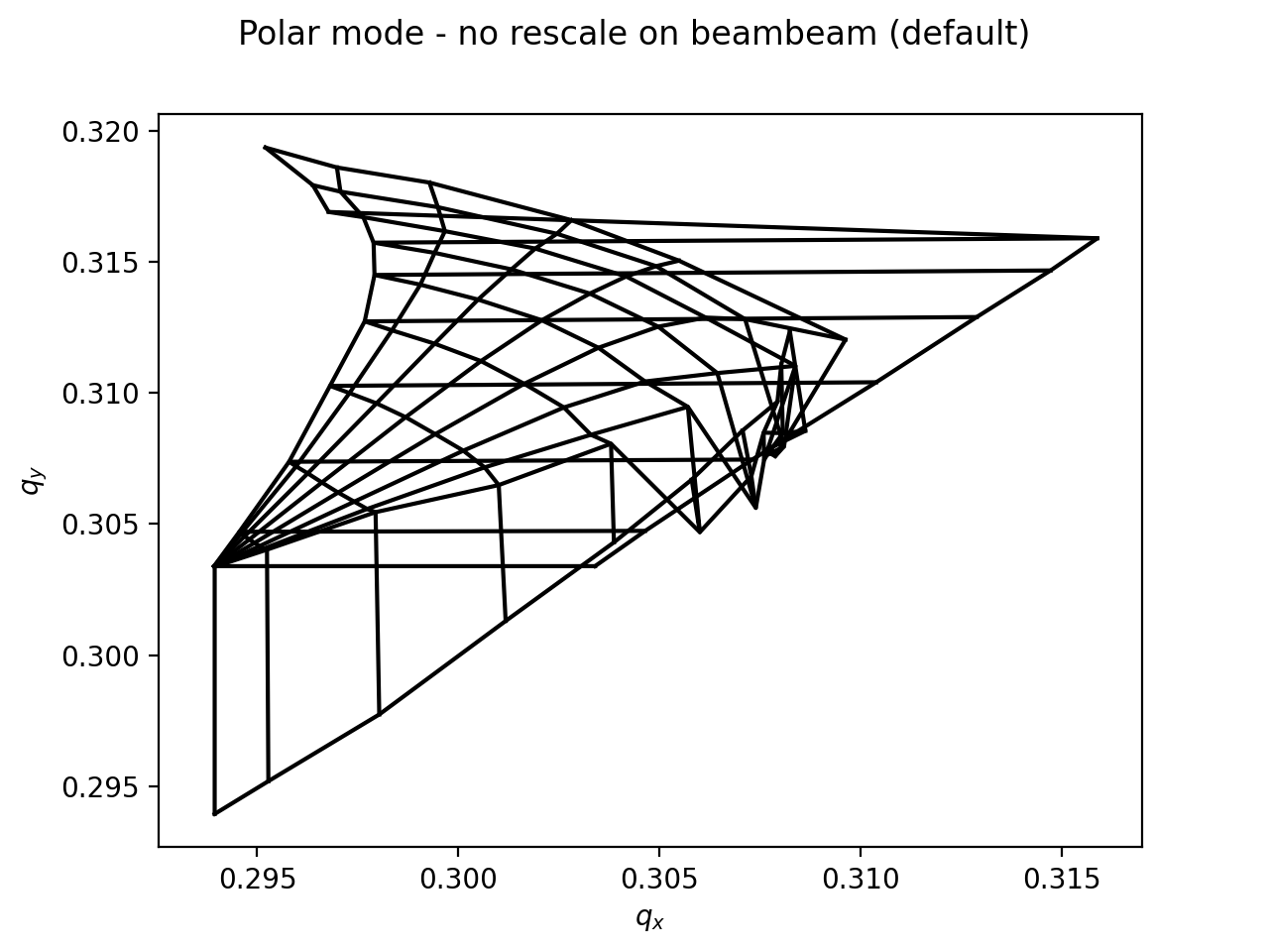
Footprints produced without rescaling beam-beam knob.
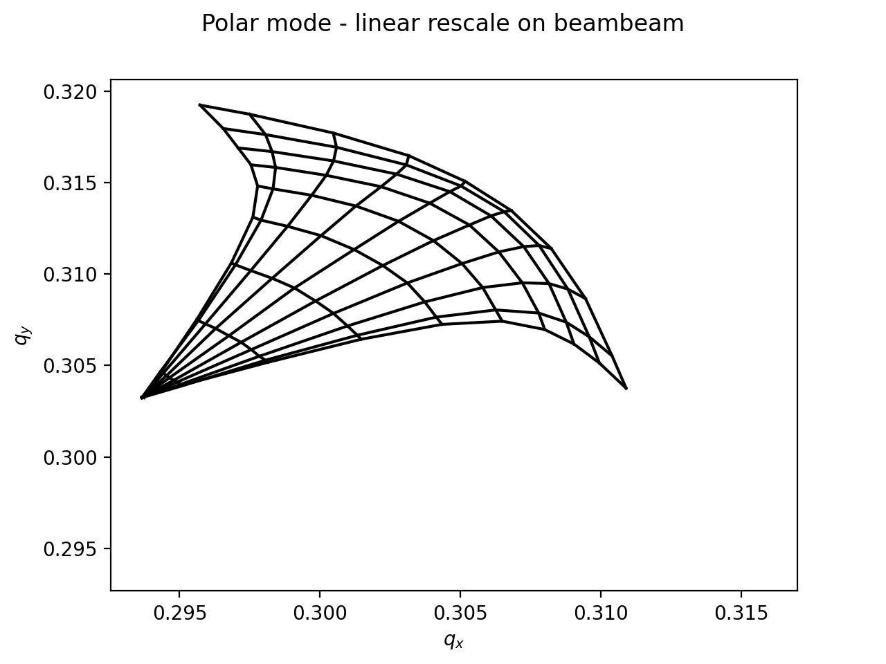
Footprints produced with rescaling beam-beam knob.
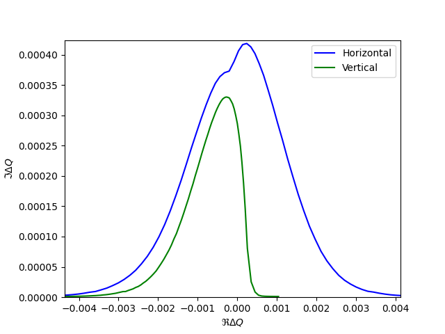
Stability diagram
Using the amplitude detuning given by the tune footprint, it is possible to evaluate numerically the dispersion integral from https://cds.cern.ch/record/318826 and obtain the stability diagram as in https://doi.org/10.1103/PhysRevSTAB.17.111002.
If the context is xobjects.ContextCupy, both the tracking and the numerical integration
are performed on the GPU.
import numpy as np
from matplotlib import pyplot as plt

import xobjects as xo
import xtrack as xt

context = xo.ContextCpu()

# ######################################### #
# Create a line with detuning               #
# and the corresponding tracker             #
# ######################################### #
Q_x = .28
Q_y = .31
Q_s = 1E-3
det_xx = 1E6
det_xy = -7E5
det_yy = -5E5
det_yx = 1E5
element = xt.LineSegmentMap(_context=context,
        qx=Q_x, det_xx = det_xx, det_xy = det_xy,
        qy=Q_y, det_yy = det_yy, det_yx = det_yx,
        qs = Q_s,bets=1.0)
line = xt.Line(elements=[element])
line.set_particle_ref('proton', p0c=7e12)

# ######################################### #
# Create footprint on a uniform grid        #
# in transverse actions Jx,Jy               #
# (given the large number of points, it     #
#  is advised not to keep the FFTs in       #
#  memory)                                  #
# ######################################### #

nemitt_x = 2.5e-6
nemitt_y = 4.5e-6
footprint = line.get_footprint(
        nemitt_x=nemitt_x, nemitt_y=nemitt_y,
        mode='uniform_action_grid',n_x_norm=200,n_y_norm=210,keep_fft=False)

# ######################################### #
# Draw the stability diagram by computing   #
# the dispersion integral for a Gaussian    #
# beam in X and Y for a set of coherent     #
# tunes with vanishing imaginary part       #
# ######################################### #

tune_shifts_x,tune_shifts_y = footprint.get_stability_diagram(context)
# ######################################### #
# Plot                                      #
# ######################################### #

plt.figure(0)
plt.plot(np.real(tune_shifts_x),np.imag(tune_shifts_x),'-b',label='Horizontal')
plt.plot(np.real(tune_shifts_y),np.imag(tune_shifts_y),'-g',label='Vertical')
plt.xlabel(r'$\Re\Delta Q$')
plt.ylabel(r'$\Im\Delta Q$')
plt.legend()
plt.show()

# Complete source: xtrack/examples/footprint/003_stability_diagram.py