Time dependent knobs

To simulate the effect of time-changing properties of the beam-line it is possible to control any lattice element attribute with a time-dependent function. For this purpose, the variable t_turn_s provides the time in seconds since the start of the simulation and is updated automatically every turn during tracking:

\[\verb|t_turn_s| = \verb|at_turn| \times \frac{L_0}{\beta_0 c_0}\]

where at_turn is the turn numer of the reference particle, \(L_0\) is the line length (design circumference), \(\beta_0\) is the relativistic beta factor of the particle tracked first and \(c_0\) is the speed of light.

The simulation of an orbit bump driven by a sinusoidal function is shown in the following example.

import numpy as np
import matplotlib.pyplot as plt

import xtrack as xt

# Build a simple ring
env = xt.Environment()
pi = np.pi
lbend = 3
line = env.new_line(components=[
    # Three dipoles to make a closed orbit bump
    env.new('d0.1',  xt.Drift,  length=0.05),
    env.new('bumper_0',  xt.Bend, length=0.05, k0=0, h=0),
    env.new('d0.2',  xt.Drift, length=0.3),
    env.new('bumper_1',  xt.Bend, length=0.05, k0=0, h=0),
    env.new('d0.3',  xt.Drift, length=0.3),
    env.new('bumper_2',  xt.Bend, length=0.05, k0=0, h=0),
    env.new('d0.4',  xt.Drift, length=0.2),

    # Simple ring with two FODO cells
    env.new('mqf.1', xt.Quadrupole, length=0.3, k1=0.1),
    env.new('d1.1',  xt.Drift, length=1),
    env.new('mb1.1', xt.Bend, length=lbend, k0=pi / 2 / lbend, h=pi / 2 / lbend),
    env.new('d2.1',  xt.Drift, length=1),
    env.new('mqd.1', xt.Quadrupole, length=0.3, k1=-0.7),
    env.new('d3.1',  xt.Drift, length=1),
    env.new('mb2.1', xt.Bend, length=lbend, k0=pi / 2 / lbend, h=pi / 2 / lbend),
    env.new('d3.4',  xt.Drift, length=1),
    env.new('mqf.2', xt.Quadrupole, length=0.3, k1=0.1),
    env.new('d1.2',  xt.Drift, length=1),
    env.new('mb1.2', xt.Bend, length=lbend, k0=pi / 2 / lbend, h=pi / 2 / lbend),
    env.new('d2.2',  xt.Drift, length=1),
    env.new('mqd.2', xt.Quadrupole, length=0.3, k1=-0.7),
    env.new('d3.2',  xt.Drift, length=1),
    env.new('mb2.2', xt.Bend, length=lbend, k0=pi / 2 / lbend, h=pi / 2 / lbend),
])
line.set_particle_ref('proton', kinetic_energy0=50e6)

# Twiss
tw = line.twiss(method='4d')

# Power the correctors to make a closed orbit bump
line['bumper_strength'] = 0.
line['bumper_0'].k0 = '-bumper_strength'
line['bumper_1'].k0 = '2 * bumper_strength'
line['bumper_2'].k0 = '-bumper_strength'

# Drive the correctors with a sinusoidal function
T_sin = 100e-6
sin = line.functions.sin
line['bumper_strength'] = (0.1 * sin(2 * np.pi / T_sin * line.ref['t_turn_s']))

# --- Probe behavior with twiss at different t_turn_s ---

t_test = np.linspace(0, 100e-6, 15)
tw_list = []
bumper_0_list = []
for tt in t_test:
    line['t_turn_s'] = tt
    bumper_0_list.append(line['bumper_0'].k0) # Inspect bumper
    tw_list.append(line.twiss(method='4d')) # Twiss

# Plot
plt.close('all')
plt.figure(1, figsize=(6.4*1.2, 4.8*0.85))
ax1 = plt.subplot(1, 2, 1, xlabel='Time [us]', ylabel='x at bump center [mm]')
ax2 = plt.subplot(1, 2, 2, xlabel='s [m]', ylabel='x [mm]')

colors = plt.cm.jet(np.linspace(0, 1, len(t_test)))

for ii, tt in enumerate(t_test):
    tw_tt = tw_list[ii]
    ax1.plot(tt * 1e6, tw_tt['x', 'bumper_1'] * 1e3, 'o', color=colors[ii])
    ax2.plot(tw_tt.s, tw_tt.x * 1e3, color=colors[ii], label=f'{tt * 1e6:.1f} us')

ax2.set_xlim(0, tw_tt['s', 'bumper_2'] + 1)
plt.subplots_adjust(left=.1, right=.97, top=.92, wspace=.27)
ax2.legend()


# --- Track particles with time-dependent bumpers ---

num_particles = 100
num_turns = 1000

# Install monitor in the middle of the bump
monitor = xt.ParticlesMonitor(num_particles=num_particles,
                              start_at_turn=0,
                              stop_at_turn =num_turns)
line.insert('monitor', monitor, at='bumper_1@start')

# Generate particles
particles = line.build_particles(
                        x=np.random.uniform(-0.1e-3, 0.1e-3, num_particles),
                        px=np.random.uniform(-0.1e-3, 0.1e-3, num_particles))

# Enable time-dependent variables
line.enable_time_dependent_vars = True

# Track
line.track(particles, num_turns=num_turns, with_progress=True)

# Plot
plt.figure(2, figsize=(6.4*0.8, 4.8*0.8))
plt.plot(1e6 * monitor.at_turn.T * tw.t_rev0, 1e3 * monitor.x.T,
         lw=1, color='r', alpha=0.05)
plt.plot(1e6 * monitor.at_turn[0, :] * tw.t_rev0, 1e3 * monitor.x.mean(axis=0),
         lw=2, color='k')
plt.xlabel('Time [us]')
plt.ylabel('x [mm]')
plt.show()

# Complete source: xtrack/examples/toy_ring/006a_dynamic_bump_sin.py

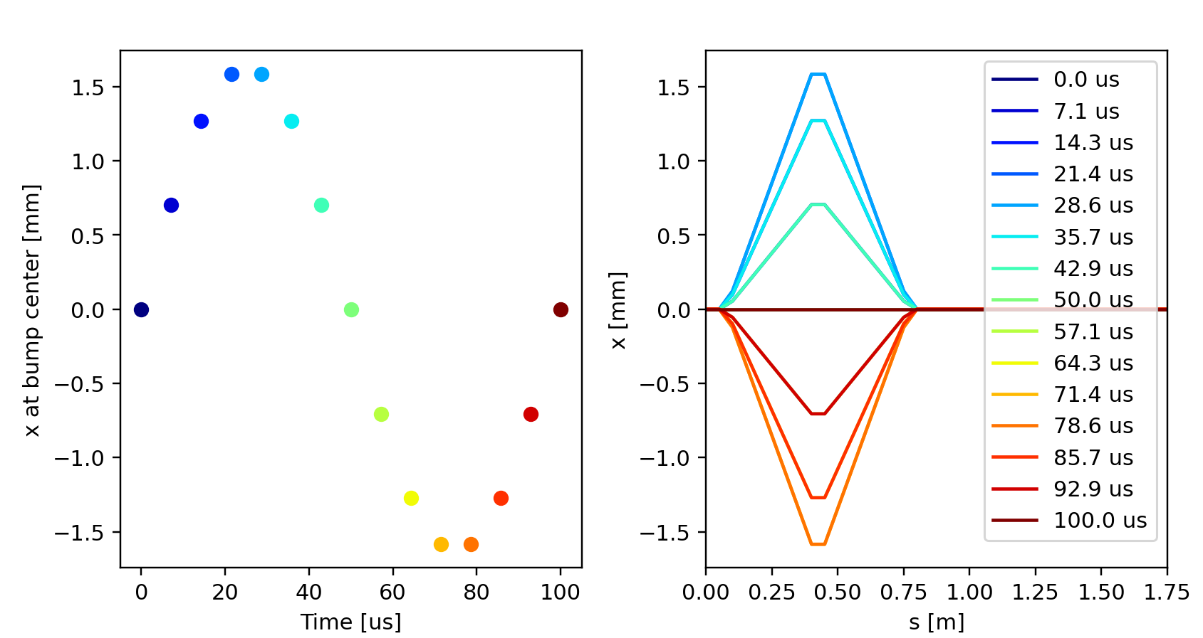
Orbit bump behavior as obained from the twiss for different settings of t_turn_s.

Beam position at the bump center during the tracking simulation. The red lines indicate the position of individual particles, the black line is their average position.

# Control the bumpers with a piece-wise linear function of time
# (outside the defined time interval, first and last point are held constant)
line.functions['my_fun'] = xt.FunctionPieceWiseLinear(
    x=np.array([10,    40,     70,   100]) * 1e-6, # time in s
    y=np.array([0,    0.5,    0.5,   1.0])        # value
)
line['bumper_strength'] = 0.1 * line.functions['my_fun'](line.ref['t_turn_s'])

# Complete source: xtrack/examples/toy_ring/006b_dynamic_bump_piece_wise_linear.py

Instead of built-in functions, it is also possible to use piece-wise linear functions defined by the user. For example, the function in the figure below can be obtained with the following code:

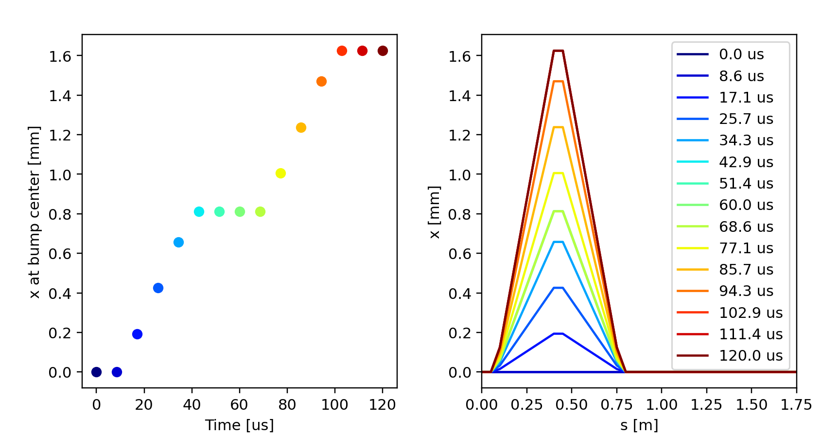
Orbit bump behavior as obained from the twiss for different settings of t_turn_s.

Beam position at the bump center during the tracking simulation. The red lines indicate the position of individual particles, the black line is their average position.

It is also possible to combine piece-wise linear functions with built-in functions in the same expression. For example, the following code can be used to generate a modulated sinusoidal function:

# Control the bumpers with a modulated sinusoidal function of time
line.functions['pulse'] = xt.FunctionPieceWiseLinear(
    x=np.array([10, 50, 150, 190]) * 1e-6, # s
    y=np.array([0,   1,   1,   0])         # knob value
)

T_sin = 10e-6
sin = line.functions.sin
line['bumper_strength'] = (0.1 * line.functions['pulse'](line.ref['t_turn_s'])
                                * sin(2 * np.pi / T_sin * line.ref['t_turn_s']))

# Complete source: xtrack/examples/toy_ring/006c_dynamic_bump_sin_env.py

Beam position at the bump center during the tracking simulation. The red lines indicate the position of individual particles, the black line is their average position.