Beam-beam
Weak-strong 2D
The example below shows how to introduce a 2D beam-beam element in a line and perform few studies based on tracking. The 2D beam-beam element provides a kick based on the Basseti-Erskine formula neglecting any longitudinal varitations of the beam-beam force.
import numpy as np
from matplotlib import pyplot as plt
import xobjects as xo
import xtrack as xt
import xfields as xf
import xpart as xp
context = xo.ContextCpu(omp_num_threads=0)
# Machine and beam parameters
n_macroparticles = int(1e4)
bunch_intensity = 2.3e11
nemitt_x = 2E-6
nemitt_y = 2E-6
p0c = 7e12
gamma = p0c/xp.PROTON_MASS_EV
physemit_x = nemitt_x/gamma
physemit_y = nemitt_y/gamma
beta_x = 1.0
beta_y = 1.0
sigma_z = 0.08
sigma_delta = 1E-4
beta_s = sigma_z/sigma_delta
Qx = 0.31
Qy = 0.32
Qs = 2.1E-3
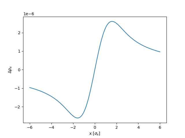
##############################
# Plot the beam-beam force #
##############################
# Particles algined on the x axis
particles = xp.Particles(_context=context,
p0c=p0c,
x=np.sqrt(physemit_x*beta_x)*np.linspace(-6,6,n_macroparticles),
px=np.zeros(n_macroparticles),
y=np.zeros(n_macroparticles),
py=np.zeros(n_macroparticles),
zeta=np.zeros(n_macroparticles),
delta=np.zeros(n_macroparticles),
)
# Definition of the beam-beam force based on the other beam's
# properties (here assumed identical to the tracked beam)
# Note that the arguments 'Sigma' are sigma**2
bbeam = xf.BeamBeamBiGaussian2D(
_context=context,
other_beam_q0 = particles.q0,
other_beam_beta0 = particles.beta0[0],
other_beam_num_particles = bunch_intensity,
other_beam_Sigma_11 = physemit_x*beta_x,
other_beam_Sigma_33 = physemit_y*beta_y)
# Build line and tracker with only the beam-beam element
elements = [bbeam]
line = xt.Line(elements=elements)
line.particle_ref = xp.Particles(mass0=xp.PROTON_MASS_EV, p0c=7e12)
line.build_tracker()
# track on turn
line.track(particles,num_turns=1)
#plot the resulting change of px
plt.figure()
plt.plot(particles.x/np.sqrt(physemit_x*beta_x),particles.px)
plt.xlabel(r'x [$\sigma_x$]')
plt.ylabel(r'$\Delta p_x$')
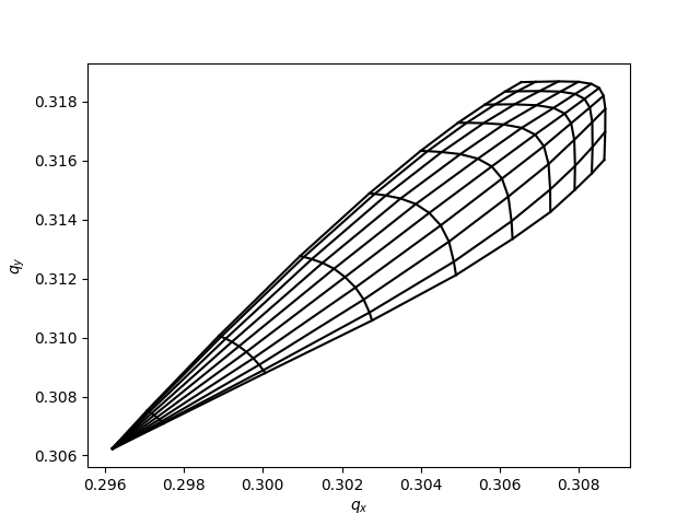
##############################
# Tune footprint #
##############################
# Build linear lattice
arc = xt.LineSegmentMap(
betx = beta_x,bety = beta_y,
qx = Qx, qy = Qy,bets = beta_s, qs=Qs)
# Build line and tracker with a beam-beam element and linear lattice
elements = [bbeam,arc]
line = xt.Line(elements=elements)
line.particle_ref = xp.Particles(mass0=xp.PROTON_MASS_EV, p0c=7e12)
line.build_tracker()
# plot footprint
plt.figure()
fp0 = line.get_footprint(nemitt_x=nemitt_x, nemitt_y=nemitt_y)
fp0.plot(color='k')
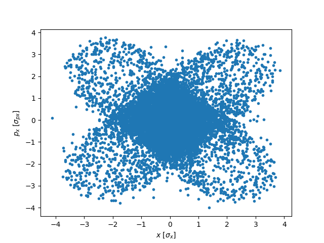
##############################
# Phase space distorion #
##############################
# Initialise particles randomly in 6D phase space
particles = xp.Particles(_context=context,
p0c=p0c,
x=np.sqrt(physemit_x*beta_x)*(np.random.randn(n_macroparticles)),
px=np.sqrt(physemit_x/beta_x)*np.random.randn(n_macroparticles),
y=np.sqrt(physemit_y*beta_y)*(np.random.randn(n_macroparticles)),
py=np.sqrt(physemit_y/beta_y)*np.random.randn(n_macroparticles),
zeta=sigma_z*np.random.randn(n_macroparticles),
delta=sigma_delta*np.random.randn(n_macroparticles),
)
# Change the tune to better visualise the 4th order resonance
arc.qx=0.255
# Track
line.track(particles,num_turns=10000)
# Plot phase space
plt.figure()
plt.plot(particles.x/np.sqrt(physemit_x*beta_x),particles.px/np.sqrt(physemit_x/beta_x),'.')
plt.xlabel('$x$ [$\sigma_x$]')
plt.ylabel('$p_x$ [$\sigma_{px}$]')
plt.show()
# Complete source: xfields/examples/002_beambeam/010_beambeam2d_weakstrong.py
Weak-strong 3D
The 3D beam-beam element can be used similarly, replacing the instanciation of the beam-beam element as in the example below. This element takes into account longitudinal variations of the beam-beam force (hourglass, crossing angle) based on a longitudinal slicing of the beam (Hirata’s method) handled by the xfields.beam_elements.TempSlicer.
# Number of longitudinal slices
n_slices = 21
# Slicer used to determine the position and charge of the slices
# based on an optimised algorithm by D. Shatilov. (other options are also possible)
slicer = xf.TempSlicer(n_slices=n_slices, sigma_z=sigma_z, mode="shatilov")
bbeam = xf.BeamBeamBiGaussian3D(
            _context=context,
            other_beam_q0 = particles.q0,
            # Full crossing angle at the IP in rad
            phi = 500.0E-2,
            # Roll angle of the crossing angle in rad (0 -> horizontal, pi/2 -> vertical)
            alpha = 0.0,
            # charge in each slice
            slices_other_beam_num_particles = slicer.bin_weights * bunch_intensity,
            # longitudinal position of the slice
            slices_other_beam_zeta_center = slicer.bin_centers,
            # transverse sizes of the slices at the IP (squarred)
            slices_other_beam_Sigma_11 = np.zeros(n_slices,dtype=float)+physemit_x*beta_x,
            slices_other_beam_Sigma_12 = np.zeros(n_slices,dtype=float),
            slices_other_beam_Sigma_13 = np.zeros(n_slices,dtype=float),
            slices_other_beam_Sigma_14 = np.zeros(n_slices,dtype=float),
            slices_other_beam_Sigma_22 = np.zeros(n_slices,dtype=float)+physemit_x/beta_x,
            slices_other_beam_Sigma_23 = np.zeros(n_slices,dtype=float),
            slices_other_beam_Sigma_24 = np.zeros(n_slices,dtype=float),
            slices_other_beam_Sigma_33 = np.zeros(n_slices,dtype=float)+physemit_y*beta_y,
            slices_other_beam_Sigma_34 = np.zeros(n_slices,dtype=float),
            slices_other_beam_Sigma_44 = np.zeros(n_slices,dtype=float)+physemit_y/beta_y)
Strong-strong (soft-Gaussian)
Strong-strong simulations can be performed using the Pipeline for multibunch simulations, as in the example below.
import time
import numpy as np
from matplotlib import pyplot as plt
from mpi4py import MPI
import xobjects as xo
import xtrack as xt
import xfields as xf
import xpart as xp
context = xo.ContextCpu(omp_num_threads=0)
####################
# Pipeline manager #
####################
# Retrieving MPI info
comm = MPI.COMM_WORLD
nprocs = comm.Get_size()
my_rank = comm.Get_rank()
# Building the pipeline manager based on a MPI communicator
pipeline_manager = xt.PipelineManager(comm)
if nprocs >= 2:
# Add information about the Particles instance that require
# communication through the pipeline manager.
# Each Particles instance must be identifiable by a unique name
# The second argument is the MPI rank in which the Particles object
# lives.
pipeline_manager.add_particles('B1b1',0)
pipeline_manager.add_particles('B2b1',1)
# Add information about the elements that require communication
# through the pipeline manager.
# Each Element instance must be identifiable by a unique name
# All Elements are instanciated in all ranks
pipeline_manager.add_element('IP1')
pipeline_manager.add_element('IP2')
else:
print('Need at least 2 MPI processes for this test')
exit()
#################################
# Generate particles #
#################################
n_macroparticles = int(1e4)
bunch_intensity = 2.3e11
physemit_x = 2E-6*0.938/7E3
physemit_y = 2E-6*0.938/7E3
beta_x_IP1 = 1.0
beta_y_IP1 = 1.0
beta_x_IP2 = 1.0
beta_y_IP2 = 1.0
sigma_z = 0.08
sigma_delta = 1E-4
beta_s = sigma_z/sigma_delta
Qx = 0.285
Qy = 0.32
Qs = 2.1E-3
#Offsets [sigma] the two beams with opposite direction
#to enhance oscillation of the pi-mode
mean_x_init = 0.1
mean_y_init = 0.1
p0c = 7000e9
print('Initialising particles')
if my_rank == 0:
particles = xp.Particles(_context=context,
p0c=p0c,
x=np.sqrt(physemit_x*beta_x_IP1)
*(np.random.randn(n_macroparticles)+mean_x_init),
px=np.sqrt(physemit_x/beta_x_IP1)
*np.random.randn(n_macroparticles),
y=np.sqrt(physemit_y*beta_y_IP1)
*(np.random.randn(n_macroparticles)+mean_y_init),
py=np.sqrt(physemit_y/beta_y_IP1)
*np.random.randn(n_macroparticles),
zeta=sigma_z*np.random.randn(n_macroparticles),
delta=sigma_delta*np.random.randn(n_macroparticles),
weight=bunch_intensity/n_macroparticles
)
# Initialise the Particles object with its unique name
# (must match the info provided to the pipeline manager)
particles.init_pipeline('B1b1')
# Keep in memory the name of the Particles object with which this
# rank will communicate
# (must match the info provided to the pipeline manager)
partner_particles_name = 'B2b1'
elif my_rank == 1:
particles = xp.Particles(_context=context,
p0c=p0c,
x=np.sqrt(physemit_x*beta_x_IP1)
*(np.random.randn(n_macroparticles)+mean_x_init),
px=np.sqrt(physemit_x/beta_x_IP1)
*np.random.randn(n_macroparticles),
y=np.sqrt(physemit_y*beta_y_IP1)
*(np.random.randn(n_macroparticles)-mean_y_init),
py=np.sqrt(physemit_y/beta_y_IP1)
*np.random.randn(n_macroparticles),
zeta=sigma_z*np.random.randn(n_macroparticles),
delta=sigma_delta*np.random.randn(n_macroparticles),
weight=bunch_intensity/n_macroparticles
)
# Initialise the Particles object with its unique name
# (must match the info provided to the pipeline manager)
particles.init_pipeline('B2b1')
# Keep in memory the name of the Particles object with which this
# rank will communicate
# (must match the info provided to the pipeline manager)
partner_particles_name = 'B1b1'
else:
# Stop the execution of ranks that are not needed
print('No need for rank',my_rank)
exit()
#############
# Beam-beam #
#############
nb_slice = 11
slicer = xf.TempSlicer(sigma_z=sigma_z, n_slices=nb_slice)
config_for_update_IP1=xf.ConfigForUpdateBeamBeamBiGaussian3D(
pipeline_manager=pipeline_manager,
element_name='IP1', # The element name must be unique and match the
# one given to the pipeline manager
partner_particles_name = partner_particles_name, # the name of the
# Particles object with which to collide
slicer=slicer,
update_every=1 # Setup for strong-strong simulation
)
config_for_update_IP2=xf.ConfigForUpdateBeamBeamBiGaussian3D(
pipeline_manager=pipeline_manager,
element_name='IP2', # The element name must be unique and match the
# one given to the pipeline manager
partner_particles_name = partner_particles_name, # the name of the
#Particles object with which to collide
slicer=slicer,
update_every=1 # Setup for strong-strong simulation
)
print('build bb elements...')
bbeamIP1 = xf.BeamBeamBiGaussian3D(
_context=context,
other_beam_q0 = particles.q0,
phi = 500E-6,alpha=0.0,
config_for_update = config_for_update_IP1)
bbeamIP2 = xf.BeamBeamBiGaussian3D(
_context=context,
other_beam_q0 = particles.q0,
phi = 500E-6,alpha=np.pi/2,
config_for_update = config_for_update_IP2)
#################################################################
# arcs (here they are all the same with half the phase advance) #
#################################################################
arc12 = xt.LineSegmentMap(
betx = beta_x_IP1,bety = beta_y_IP1,
qx = Qx/2, qy = Qy/2,bets = beta_s, qs=Qs/2)
arc21 = xt.LineSegmentMap(
betx = beta_x_IP1,bety = beta_y_IP1,
qx = Qx/2, qy = Qy/2,bets = beta_s, qs=Qs/2)
#################################################################
# Tracker #
#################################################################
# In this example there is one Particles object per rank
# We build its line and tracker as usual
elements = [bbeamIP1,arc12,bbeamIP2,arc21]
line = xt.Line(elements=elements)
line.build_tracker()
# A pipeline branch is a line and Particles object that will
# be tracked through it
branch = xt.PipelineBranch(line, particles)
# The multitracker can deal with a set of branches (here only one)
multitracker = xt.PipelineMultiTracker(branches=[branch])
#################################################################
# Tracking (Same as usual) #
#################################################################
print('Tracking...')
time0 = time.time()
nTurn = 1024
multitracker.track(num_turns=nTurn,turn_by_turn_monitor=True)
print('Done with tracking.',(time.time()-time0)/1024,'[s/turn]')
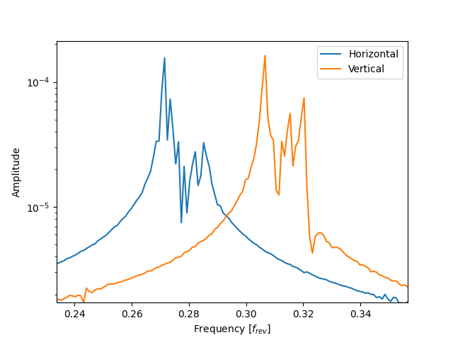
#################################################################
# Post-processing: raw data and spectrum #
#################################################################
# Show beam oscillation spectrum (only one rank)
if my_rank == 0:
positions_x_b1 = np.average(line.record_last_track.x,axis=0)
positions_y_b1 = np.average(line.record_last_track.y,axis=0)
plt.figure(1)
freqs = np.fft.fftshift(np.fft.fftfreq(nTurn))
mask = freqs > 0
myFFT = np.fft.fftshift(np.fft.fft(positions_x_b1))
plt.semilogy(freqs[mask], (np.abs(myFFT[mask])),label='Horizontal')
myFFT = np.fft.fftshift(np.fft.fft(positions_y_b1))
plt.semilogy(freqs[mask], (np.abs(myFFT[mask])),label='Vertical')
plt.xlabel('Frequency [$f_{rev}$]')
plt.ylabel('Amplitude')
plt.legend(loc=0)
plt.show()
# Complete source: xfields/examples/002_beambeam/006_beambeam6d_strongstrong_pipeline_MPI2Procs.py
In collisions featuring a low disruption (i.e. the beam moments do not vary significantly during the interaction), the quasi-strong-strong (aka frozen-strong-strong) model may be enabled by setting the argument ‘quasistrongstrong
= True’ in xfields.beam_elements.ConfigForUpdate*. In this configuration, the beam moments are computed once at the start of the collison and kept constant throught the collison, thus reducing the computing load. The argument ‘update_every’ allows to further reduce the computing load by keeping the moments for the given amount of turns. This model is suitable for effects that build up over may turns. (more details in https://accelconf.web.cern.ch/eefact2022/papers/wezat0102.pdf)
For a 2D beam-beam interactions, the beam-beam element and the xfields.beam_elements.ConfigForUpdate* have to be redifined as in the example below.
config_for_update_b1_IP1=xf.ConfigForUpdateBeamBeamBiGaussian2D(
   pipeline_manager=pipeline_manager,
   element_name='IP1',
   partner_particles_name = 'B2b1',
   update_every=1
   )
config_for_update_b2_IP1=xf.ConfigForUpdateBeamBeamBiGaussian2D(
   pipeline_manager=pipeline_manager,
   element_name='IP1',
   partner_particles_name = 'B1b1',
   update_every=1
   )
bbeamIP1_b1 = xf.BeamBeamBiGaussian2D(
            _context=context,
            other_beam_q0 = particles_b2.q0,
            other_beam_beta0 = particles_b2.beta0[0],
            config_for_update = config_for_update_b1_IP1)
bbeamIP1_b2 = xf.BeamBeamBiGaussian2D(
            _context=context,
            other_beam_q0 = particles_b1.q0,
            other_beam_beta0 = particles_b1.beta0[0],
            config_for_update = config_for_update_b2_IP1)
Poisson Solver
Particle-in-cell simulations using a Poisson solver for the beam-beam interaction is currently not implemented in xfields
Beam-beam in a real lattice
Identically to the examples above, beam-beam elements can be introduced into the lattice of a full machine. Several tools exist to ease the setup of beam-beam interactions in a collider lattice: Xmask. An example snippet is shown below where an xtrack lattice in json format is loaded and a weakstrong beam-beam element is inserted at the marker “ip.1”.
path     = "/path/to/lattice"
seq_name = "lattice.json"
seq_path = os.path.join(path, seq_name)

 with open(seq_path, 'r') as f:
     line = xt.Line.from_dict(json.load(f))

# define slicer
slicer = xf.TempSlicer(n_slices=n_slices, sigma_z=sigma_z, mode=binning_mode)

# define weakstrong beambeam element (n*[x] yields a list with n elements each of which is x, e.g. 3*[5]=[5,5,5])
el_beambeam = xf.BeamBeamBiGaussian3D(
         _context=context,
         config_for_update = None,
         other_beam_q0=other_beam_q0,
         phi=phi, # half-crossing angle in radians
         alpha=alpha, # crossing plane in radians
         # slice intensity [num. real particles] number of slices inferred from the length of this list
         slices_other_beam_num_particles = slicer.bin_weights * nb,
         # unboosted opposing (strong) beam moments
         slices_other_beam_zeta_center = slicer.bin_centers,
         slices_other_beam_Sigma_11    = n_slices*[ sigma_x**2], # Beam sizes for the other beam, assuming the same value for all slices
         slices_other_beam_Sigma_22    = n_slices*[sigma_px**2],
         slices_other_beam_Sigma_33    = n_slices*[ sigma_y**2],
         slices_other_beam_Sigma_44    = n_slices*[sigma_py**2],
         # only if beamstrahlung on
         slices_other_beam_zeta_bin_width_star_beamstrahlung = None if not beamstrahlung_on else slicer.bin_widths_beamstrahlung / np.cos(phi),  # boosted dz
         # has to be set (0 in most cases) if config_for_update = None
         slices_other_beam_Sigma_12     = n_slices*[0],
         slices_other_beam_Sigma_34     = n_slices*[0],
         slices_other_beam_pzeta_center = n_slices*[pzeta], # important when tapering (FCC-ee specific)
     )

element_name = "ip.1"  # this is the marker name of an IP in the lattice where the beam-beam element will be inserted
element_line_index = line.element_names.index(element_name)  # get the array index of the element "ip.1"
line.insert_element(index=element_line_index, element=el_beambeam, name='beambeam')