Acceleration
An energy ramp with an arbitrary time dependence of the beam energy can be
simulated by attaching and xtrack.EnergyProgram object to the line, as
shown in the example below.
import numpy as np
from cpymad.madx import Madx
import xtrack as xt

# Import a line and build a tracker
line = xt.Line.from_json(
    '../../test_data/psb_injection/line_and_particle.json')
e_kin_start_eV = 160e6
line.particle_ref = xt.Particles(mass0=xt.PROTON_MASS_EV, q0=1.,
                                 energy0=xt.PROTON_MASS_EV + e_kin_start_eV)
line.build_tracker()

# User-defined energy ramp
t_s = np.array([0., 0.0006, 0.0008, 0.001 , 0.0012, 0.0014, 0.0016, 0.0018,
                0.002 , 0.0022, 0.0024, 0.0026, 0.0028, 0.003, 0.01])
E_kin_GeV = np.array([0.16000000,0.16000000,
    0.16000437, 0.16001673, 0.16003748, 0.16006596, 0.16010243, 0.16014637,
    0.16019791, 0.16025666, 0.16032262, 0.16039552, 0.16047524, 0.16056165,
    0.163586])

# Attach energy program to the line
line.energy_program = xt.EnergyProgram(t_s=t_s, kinetic_energy0=E_kin_GeV*1e9)

# Plot energy and revolution frequency vs time
t_plot = np.linspace(0, 10e-3, 20)
E_kin_plot = line.energy_program.get_kinetic_energy0_at_t_s(t_plot)
f_rev_plot = line.energy_program.get_frev_at_t_s(t_plot)

import matplotlib.pyplot as plt
plt.close('all')
plt.figure(1, figsize=(6.4 * 1.5, 4.8))
ax1 = plt.subplot(2,2,1)
plt.plot(t_plot * 1e3, E_kin_plot * 1e-6)
plt.ylabel(r'$E_{kin}$ [MeV]')
ax2 = plt.subplot(2,2,3, sharex=ax1)
plt.plot(t_plot * 1e3, f_rev_plot * 1e-3)
plt.ylabel(r'$f_{rev}$ [kHz]')
plt.xlabel('t [ms]')

# Setup frequency of the RF cavity  to stay on the second harmonic of the
# revolution frequency during the acceleration

t_rf = np.linspace(0, 3e-3, 100) # time samples for the frequency program
f_rev = line.energy_program.get_frev_at_t_s(t_rf)
h_rf = 2 # harmonic number
f_rf = h_rf * f_rev # frequency program

# Build a function with these samples and link it to the cavity
line.functions['fun_f_rf'] = xt.FunctionPieceWiseLinear(x=t_rf, y=f_rf)
line.element_refs['br.c02'].frequency = line.functions['fun_f_rf'](
                                                        line.vars['t_turn_s'])

# Setup voltage and lag
line.element_refs['br.c02'].voltage = 3000 # V
line.element_refs['br.c02'].lag = 0 # degrees (below transition energy)

# When setting line.vars['t_turn_s'] the reference energy and the rf frequency
# are updated automatically
line.vars['t_turn_s'] = 0
line.particle_ref.kinetic_energy0 # is 160.00000 MeV
line['br.c02'].frequency # is 1983931.935 Hz

line.vars['t_turn_s'] = 3e-3
line.particle_ref.kinetic_energy0 # is 160.56165 MeV
line['br.c02'].frequency # is 1986669.0559674294

# Back to zero for tracking!
line.vars['t_turn_s'] = 0

# Track a few particles to visualize the longitudinal phase space
p_test = line.build_particles(x_norm=0, zeta=np.linspace(0, line.get_length(), 101))

# Enable time-dependent variables (t_turn_s and all the variables that depend on
# it are automatically updated at each turn)
line.enable_time_dependent_vars = True

# Track
line.track(p_test, num_turns=9000, turn_by_turn_monitor=True, with_progress=True)
mon = line.record_last_track

# Plot
plt.subplot2grid((2,2), (0,1), rowspan=2)
plt.plot(mon.zeta[:, -2000:].T, mon.delta[:, -2000:].T, color='C0')
plt.xlabel(r'$\zeta$ [m]')
plt.ylabel('$\delta$')
plt.xlim(-40, 30)
plt.ylim(-0.0025, 0.0025)
plt.title('Last 2000 turns')
plt.subplots_adjust(left=0.08, right=0.95, wspace=0.26)
plt.show()

# Complete source: xtrack/examples/acceleration/001_energy_ramp.py
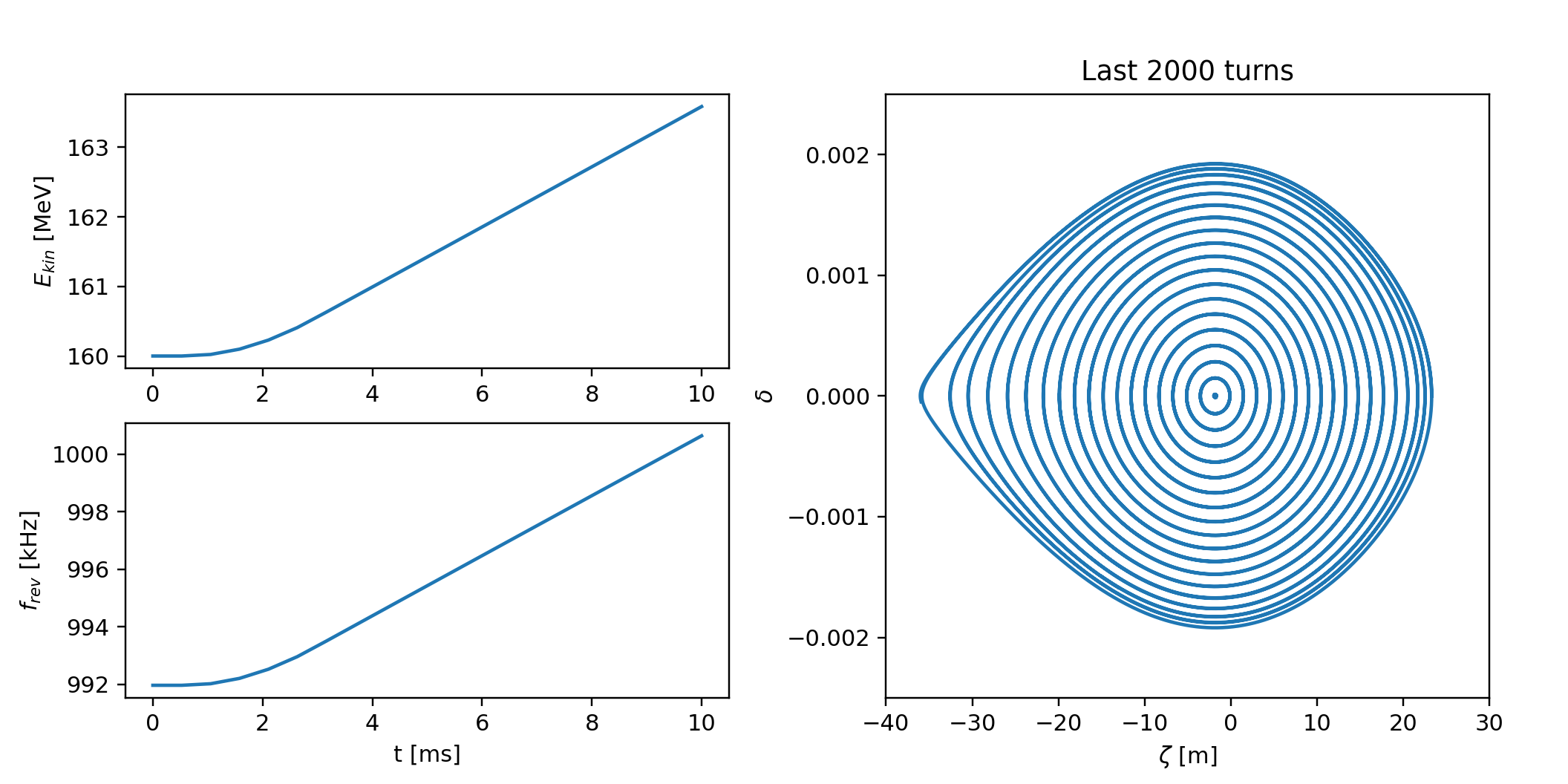
Time evolution of the beam energy and the RF frequency and particles motion in the longitudinal phase space as obtained from the example above.